


 Inglês (pdf)
 Artigo em XML
 Referências do artigo

 Permalink
1. Introduction
Livestock farming plays a vital role in supporting the sustenance and economic livelihood of more than 1.3 billion people. By utilizing land unsuitable for traditional crop cultivation, it constitutes the largest single land use, contributing to 17% of the world's total energy intake through food products1. Despite these substantial contributions, the livestock sector is increasingly under scrutiny for its environmental impact2, and it is also encountering growing competition for land3 and labor resources.
In a context where projections anticipate ongoing growth in beef demand4, the opportunity to enhance livestock productivity becomes clear. This enhancement is essential not only for stimulating economic development but also for mitigating environmental impacts, boosting the competitiveness of cattle farms, increasing overall food production, and fulfilling environmental commitments.
In the global context, Uruguay stands out as a crucial case study due to its longstanding tradition in the global beef export market. Data from the latest agricultural census in 2011 reveal that meat and milk livestock farming served as the primary source of income for 74% of commercial agricultural farms. This sector occupies a vast expanse, encompassing 12.6 million hectares, which constitute 70% of the national territory.
Historically, Uruguay's beef production has thrived due to its cost-effective natural field grazing system, providing the country with a unique competitive advantage that endures to this day. However, the beef production growth in Uruguay has not kept pace with other sectors like forestry, agriculture, and dairy5. This challenge is further complicated by the fact that, over the past two decades, the evolution of beef production per hectare in Uruguay has exhibited fluctuations without a clear trend 6)(7)8)(9) . A more comprehensive understanding of livestock farming underscores the importance of investigating the heterogeneity in production at the ranch level, as this is where farmers make the decisions. Various factors unique to each farming operation process, including cattle focus, local weather conditions, management practices, and resource availability, significantly influence beef production.
In Uruguay, a stark contrast exists in the performance of different cattle ranches. The top 10% of ranches produce five times more beef per hectare compared to the bottom 10% 10)(11) . However, these fluctuations in yield alone do not capture the variations in input utilization intensities and other inherent attributes of beef production. Hence, they may not be suitable indicators for comparing the performance of different ranches. To address this issue, the study suggests estimating the farm-level technical efficiency (TE hereafter) as an indicator of the production unit's management capability.
TE is a comparative concept that measures the proportion of actual production observed relative to the maximum potential production attainable, while taking into account factors such as resource availability, input utilization, and available technology. In simpler terms, TE serves as an advanced performance metric, assessing how effectively a production unit transforms inputs into outputs within the constraints of available technology.
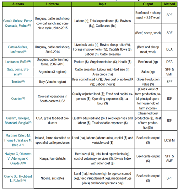
Table S1 in the Supplementary material compiles prior research endeavors focused on estimating technical efficiency within beef cattle farming at the farm level, spanning diverse geographic and operational contexts, providing valuable insights into the efficiency of beef cattle farming. Nevertheless, making direct comparisons between these studies is challenging due to variations in the methodologies employed, target populations, and contextual factors. For instance, Trestini12 used a stochastic production frontier model to evaluate TE using an unbalanced panel of beef cattle farms in Veneto, Italy, reporting an average farm TE of 0.786. Qushim and others13 delved into scale and technical efficiency in cow-calf farms in the Southeastern United States, employing an input distance function analysis to evaluate economic performance based on gross value of farm production and total principal operator household off-farm income, uncovering an average efficiency of 0.86. Otieno and others14) estimated TE levels in Kenyan beef cattle production across various systems, including nomads, agro-pastoralists, and ranchers, using a stochastic metafrontier, resulting in an average TE of 0.69.
Furthermore, Gatti and others15 applied a meta-frontier methodology to assess TE and technology disparities in beef cattle production across distinct regions in Argentina, finding that they could not reject the hypothesis of constant returns to scale but did reject the null hypothesis that the regions shared the same technology. Nwigwe and others16 measured the TE of nomadic pastoralists, agro-pastoralists, and ranchers in six Nigerian states using a separated stochastic production frontier, finding average TEs of 0.59, 0.69, and 0.83 for the three groups, respectively. Additionally, Qushim and others17 delved into TEs in U.S. grass-fed beef production through a stochastic input distance function with two outputs (whole farm and grass-fed beef enterprise), revealing average TEs of 0.84 for whole farms and 0.79 for enterprises within the U.S. grass-fed beef sector. Lastly, Martinez-Cillero and others18 used a latent class stochastic frontier model with an unbalanced panel of Irish farmers to assess TE, focusing on TE in farms classified as specialist cattle producers, and their findings indicate that a single frontier model tends to overestimate technical inefficiency compared to a model that considers technology heterogeneity.
In the Uruguayan context, prior estimations of technical efficiency have relied on private records from ranches associated with technical assistance entities. Lanfranco and Buffa19 applied the Data Envelopment Analysis technique and revealed that 6 out of the 27 studied companies engaged in beef cattle fattening were efficient. Similarly, García-Suárez and Lanfranco20 employed the Data Envelopment Analysis technique to examine beef cattle farms, yielding an average TE of 0.772. Additionally, García-Suárez and others21 used both a stochastic production frontier with one combined output (equivalent meet) and a stochastic ray frontier with three outputs (beef, sheep-meat and wool), reporting average TE levels of 0.769 and 0.779, respectively.
However, these prior studies, despite their valuable contributions, were limited in their sample coverage, preventing them from providing a comprehensive overview of the TE representative of the entire sector at the national level. This is the primary contribution of our study. To achieve this, we utilize data from the last General Agricultural Census of 2011, which have not been previously utilized for this purpose.
The focus of this article is on ranchers engaged with cow-calf production, primarily involved in cattle grazing, and having more than seven bovine livestock units and over 50 hectares of pasture. Dairy farms and ranches specializing in finishing are intentionally excluded from our target population. As a result, our analysis significantly enhances the accuracy, representativeness, and comprehensiveness of the study, encompassing the entire beef industry in Uruguay with cow-calf production.
While the snapshot presented by the data from the last General Agricultural Census of 2011 may not fully capture the technological landscape of the entire Uruguayan livestock industry, it serves as a valuable point of comparison for cow-calf producers. Moreover, the estimates obtained from this study can be used as a reference point for comparing the data from the upcoming General Agricultural Census 2022, which is currently in progress.
In this study, we aim to address two pivotal research questions: 'How can we comprehensively assess and quantify the technical efficiency (TE) of individual ranches in Uruguay's beef cattle farming sector using census data?', and 'Which variables have a significant impact on TE in Uruguay's beef cattle farming industry?' By addressing these questions, our objective is to provide insights that are pertinent for public policy analysis, offering the potential to inform the design, targeting, monitoring, and evaluation of evidence-based policies within the industry.
We employed a stochastic translog production function approach based on Wang's model22 to estimate beef production efficiency. This estimation was conducted through cross-sectional data analysis, incorporating three primary inputs: equivalent bovine units, grazing area, and equivalent workers. Additionally, we integrated several control variables into our analysis, including region, on-site infrastructure and improvements, soil suitability for livestock, the proportion of land undergoing forage improvements, and technological orientation.
We also included additional variables to help in interpreting both the expected values and the variance linked to inefficiency. These variables encompass aspects such as the availability of technical assistance in agronomy, veterinary medicine, and accounting; the proportion of cattle owned by third parties; the extent of reliance on livestock farming as the primary source of income, and the utilization of outsourced services.
In our study, we observed a simple average TE of 76.2% among the ranches. When we applied weights to the data by farm size, this average TE increased to 79.1%. Our findings emphasized that factors such as the primary source of income originating from the farm, the utilization of third-party services, the proportion of foreign-owned cattle, and the utilization of agronomic and veterinary technological advice have a significant impact on TE.
This study represents a pioneering effort in utilizing national-level administrative records, including data from the most recent General Agricultural Census and the National Livestock Information System, to estimate TE in Uruguay's beef cattle farming sector. By providing a comprehensive and representative analysis covering the entire beef industry in Uruguay, this research aims to illuminate variations in efficiency at the ranch level, identify significant factors contributing to TE, and offer actionable insights for policy considerations aimed at promoting sustainable development and competitiveness. The findings provide valuable insights for policymaking that align with the nation's economic and environmental objectives, including the goal of reducing emission intensity measured as emissions per gross product23.
2. Materials and methods
2.1 Data sources
In this study, we have integrated data from Uruguay's most recent General Agricultural Census (CGA, for its Spanish acronym) with records from the National Livestock Information System (SNIG, for its Spanish acronym), which is Uruguay's livestock traceability system. The CGA24, although it is based on data from 2011, offers a comprehensive overview of all agricultural ranches in the country. On the other hand, the SNIG is mandatory for all livestock owners and tracks the temporal and spatial dynamics of various species, including bovine, ovine, swine, equine, and goat. This system combines annual stock declarations (as of June 30) with all associated changes in livestock ownership or location.
By merging these datasets at the farm level10, we define a farm as the unit of analysis in the census data. Then, a farm is represented by an aggregation of plots unified by shared production factors and management. This combined dataset enables us to measure production and performance on a granular, farm-by-farm basis across the country. While the agricultural year data from the 2011 census may appear out of date, it remains as an invaluable benchmark, offering insights into the intricacies and changes within the livestock sector.
2.2 Method
To measure technical efficiency (TE), we used the output increasing oriented indicator proposed by Farrel25, contrasting the observed output of a farm with the potential output of a fully efficient farm using the same inputs and technology.
The Stochastic Production Frontier (SPF) approach can be viewed as a generalization of the classical production model. In this approach, the efficiency of resources is considered as an empirical constraint to be tested, rather than an a priori assumption of neoclassical production theory26. For recent literature on this topic, refer to Kumbhakar and others 27)(28) 29, and Sickles and Zelenyuk26.
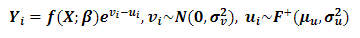
Let 70. Y 71. 𝑖 72. represent the output of production unit 𝑖, 73. 𝑋 74. 𝑖 75. an input vector of dimension K, and 76. 𝑓(𝑋 77. 𝑖 78. ;𝛽) the production function. We introduce 79. 𝑢 80. 𝑖 81. as a non-negative error following the distribution 82. 𝐅 83. + 84. ( 85. 𝛍 86. 𝐮 87. , 88. 𝛔 89. 𝐮 90. 𝟐 91. ), and 92. 𝑣 93. 𝑖 94. a symmetric normal error. While 95. 𝑣 96. 𝑖 97. accounts for elements such as measurement error, specification issues, and random variability in the production process, 98. 𝑢 99. 𝑖 100. represents technical inefficiency that reduces the observed output level relative to its potential.
The SPF for cross-sectional data can be expressed as:
To estimate this equation parametrically, it is necessary to specify f(Xi ; β), which we assume to be a translog functional form due to its flexibility27:
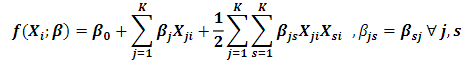
The functional form described facilitates the derivation of product input elasticities and accommodates non-constant returns to scale. Specifically, when all coefficients tied to second-degree terms ( 110. 𝛽 111. 𝒋𝒔 112. ) are zero, the Cobb-Douglas function emerges as a subset. It's worth noting that the translog and Cobb-Douglas functions can be conceptualized as the second and first-order Taylor series approximations of a broader production function, respectively27.
Additionally, it is necessary to assume the distribution of the technical inefficiency term ( 114. 𝑢 115. 𝑖 116. ), which, by definition, can only take positive values. The model developed by Wang22 assumes that there is a set of exogenous variables Z that affects the mean and the variance of technical inefficiency, and it is assumed to be positive truncated normal:
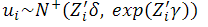
Wang's model encompasses several specific cases. These include the Half Normal30 and Truncated Normal31 (TN) specifications, which do not incorporate contextual variables. There are also variations such as the Kumbhakar, Ghosh and McGuckin32 (KGM) model, which parameterizes the distribution mean of inefficiency with exogenous variables, and the Caudill and Ford33 (CF) model, which parameterized the variance.
Additionally, we include control variables in the production frontier to account for variations in technological orientation among livestock ranches, natural soil suitability, the utilization of forage enhancements, and spatial production disparities. Therefore, the equation to be estimated, which includes a vector of control variables 122. 𝑪 123. 𝒊 124. with a vector of coefficients 125. 𝜃 126. 𝑻 127. , is as follows:
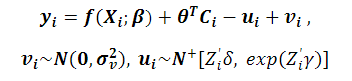
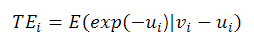
To estimate the likelihood of the model, it is assumed that the distribution of the random variables 132. 𝑢 133. 𝑖 134. and 135. 𝑣 136. 𝑖 137. is independent, conditional on ( 138. 𝑋 139. 𝑖 140. , 141. 𝑍 142. 𝑖 143. ). The estimation of all the model parameters is carried out in a single stage using the maximum likelihood method. In a second stage, the estimation of TE is derived, using the conditional distribution of 144. 𝑢 145. 𝑖 146. | 147. 𝑣 148. 𝑖 149. :
Implicitly, the model assumes exogeneity of all inputs, which implies the absence of unobservable producer-level heterogeneity that could account for variations in input utilization.
To test the hypotheses on the model restrictions, the likelihood ratio test is employed, expressed as
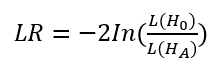
Where L(Ho) and L(H A ) represent the likelihood under the null and alternative hypothesis, respectively. The LR statistic asymptotically follows a chi-square distribution with J degrees of freedom.
Finally, to explore the heterogeneity in TE across farms, we employed a tree-based algorithm to group the farms34. This approach allows for a flexible modeling of the relationship between TE and a set of explanatory variables without imposing restrictive assumptions about the functional form. Specifically, we employed a Conditional Inference Tree35 (CTREE) regression for this purpose. Tree-type models iteratively divide the explanatory variable space, optimizing the dependent variable (TE). The CTREE determines the significance of each partition based on the strength of the association between the explanatory variable and the target variable, using non-parametric tests to test all possible associations. It is important to note that these results are exploratory and should not be interpreted causally36.
2.3 Empirical strategy
The target population of this article comprises ranchers with cow-calf production, with a minimum production scale (more than 50 grazing hectares and 7 livestock units), and a specific focus in cattle grazing. To reduce the heterogeneity of production systems, we have excluded the following categories: dairy farms, ranches specialized in sheep production, cattle breeders, feedlots, and ranches specialized in fattening. These exclusions are intended to simplify the complexity of beef farming and approximate it through a production function focused on a single composite product. This simplification aids in mapping inputs to products and modeling the technology.
After defining our target population and assessing the quality of the livestock census forms (see the appendix in the Supplementary materials for details), our sample comprises 5,057 farms, collectively managing more than 3.7 million hectares of land and 3 million animals.
In this analysis, we have included farms owned by corporations. This inclusion requires the exclusion of certain explanatory variables for technical efficiency that are only available for farms owned by individuals (e.g., age, sex, educational level, residing on the farm).
The variables used to model beef production are based on previous studies (see Table S1) and the available information in our database. The chosen output variable to characterize beef cattle farming is the production of live cattle meat in the livestock year 2011/2012 (in kg). The computation of meat production at the livestock farm level is based on the net difference between sales and purchases, accounting for inventory changes due to events such as births, deaths, and category changes resulting from animal growth. Sales are categorized into two primary types: the sale of fattened cattle intended for slaughter, and the exchange of lean cattle among producers. The details to compute beef production are described in Aguirre9.
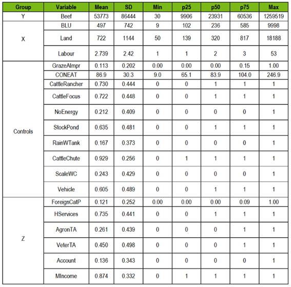
The inputs of production encompass the products and services employed in the beef cattle production process, including materials, labor, and capital. These inputs must satisfy specific criteria: they should be essential, show a positive monotonic relationship with the output, and be divisible. The inputs considered in the analysis are: (1) bovine animals measured in bovine livestock units (BLU); (2) LAND area devoted to beef cattle production; (3) total LABOR force in the farm, calculated as the sum of permanent workers plus the number of hired daily laborers in the year divided by 250 (total work days in a year).
In Uruguay, a BLU represents the energy requirements of a cow of 380 kg of live weight in maintenance. An equivalence system is widely used, assigning different categories of cattle a coefficient that weighs their relative consumption compared to that of the standard BLU.
To address the heterogeneity in livestock farming, the production function includes a set of control variables: (1) forage production capacity, represented by the natural productivity of soil for cattle production using the CONEAT index, and the proportion of area with forage improvements; (2) technological orientation, distinguishing between cattle ranchers or mixed operations, and those engaged in cow-calf or complete cycle production; (3) ranch infrastructure, encompassing amenities such as electricity, water reservoirs, rainwater tanks, private vehicles, cattle weighing chutes, and cattle scales; and (4) geographical factors, captured by 18 dummy variables representing each region (department in Uruguay), excluding Montevideo.
The CONEAT index was developed by the Uruguayan government to measure the production capacity of land in terms of meat and wool and the land units that comprise it. The index is used for fiscal purposes, has an average value of 100 at the national level, and ranges from 0 (land not suitable for livestock) to a maximum of 250.
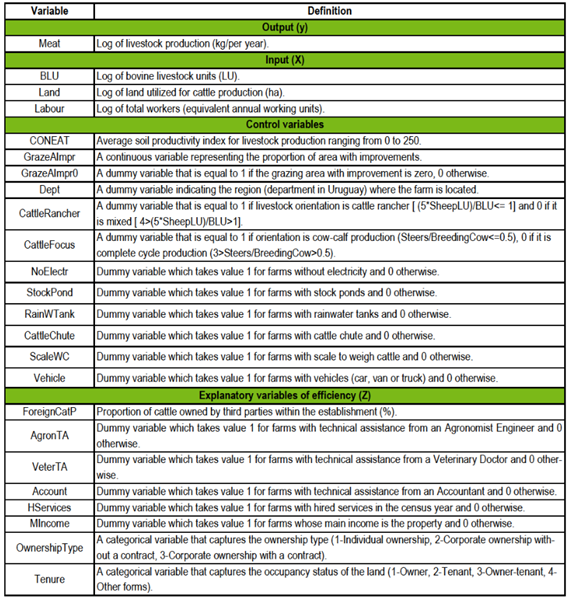
The ratio of area with improvements represents the proportion of the soil that has enhancements over natural grass, allowing for greater forage capacity, and therefore, the potential to feed more cattle. The greater the proportion of improved area, the higher the expected forage capacity, and, consequently, a greater potential to sustain more livestock.
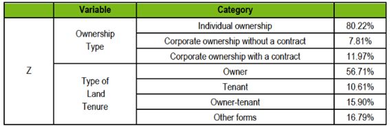
Lastly, a set of explanatory variables Z is introduced to consider factors that potentially affect efficiency. While these variables do not influence the production possibilities frontier, they can impact the distance between the evaluated farm and the frontier. The explanatory variables consist of: (1) the utilization of services and technical assistance (agronomic, veterinary, and accounting); (2) the type of land tenure; (3) the type of ownership of the ranch; (4) the proportion of livestock owned by others, and (5) the importance of beef production in the family's income.
All the variables used in this study are expressed in physical units rather than monetary values. This approach enables us to account for price fluctuations, eliminating the need for substantial assumptions about resource prices or opportunity costs.
When calculating descriptive statistics for the output and input variables (Table S2 and Table S3 in the Supplementary material), we observe significant heterogeneity in terms of the range of variation, the interquartile range (p75-p25), and the coefficient of variation (S.D/Mean). For example, the coefficient of variation is 1.61 for bovine meat, 1.49 for bovine livestock units, 1.58 for land area, and 0.88 for labor. As expected, there is a strong linear correlation between meat production (output) and the inputs. The Pearson correlation coefficient for bovine meat with bovine livestock units is 0.948, with land area it is 0.899, and with the number of workers it is 0.741.
3. Results
3.1 The beef production model
This section presents the results of the models for the 5,057 livestock farms in the sample that meet our study universe's definition. The estimations were performed using the sfcross package in the STATA software37.
The Wang translog specification allows us to test hypotheses by comparing it with alternative models as special cases (see Table S4 in the Supplementary material). Firstly, we reject the hypothesis ( 192. 𝐻 193. 01 194. ) that the Cobb-Douglas functional form is preferred over the translog alternative (pv < 0.1%). We also reject the hypothesis of the absence of technical inefficiency ( 195. 𝐻 196. 05 197. ). Next, we contrast whether the Wang model is preferred over the alternative without explanatory variables for inefficiency (Wang vs. TN), with explanatory variables parameterized only at the mean (Wang vs. KGM), and with explanatory variables parameterized only at the variance (Wang vs. CF). All three alternatives are rejected (pv < 0.1%). Therefore, from now on, we will provide a detailed discussion of the results of the Wang translog specification.
Figure 1 displays the 95% confidence intervals (CI) for the input-output elasticities, evaluated at the mean values of the inputs. A 1% increment in BLU, LAND, and LABOUR leads to an average increase in meat production of 0.789%, 0.164%, and 0.03% respectively, all statistically significant at the 5% level.
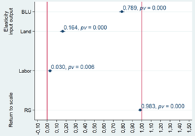
Figure 1: 95% confidence intervals for input-output elasticities and returns to scale, all evaluated at the mean value (BLU=497, LAND=722, LABOUR=2.79)
The response of elasticity is not uniform across the inputs’ support (Figure 2): BLU's impact increases up to 400 and then levels off; LAND's effect declines until 500 and then stabilizes at a value beneath the average elasticity; LABOUR's influence shows no significant deviation from the mean value throughout the observed range.
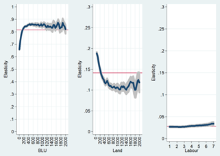
The study reveals an average return to scale of 0.983, which is statistically indistinguishable from 1 (p-value of 0.142), indicating constant returns to scale. A closer look at the entire input range (Figure 3) reveals no substantial deviations from this scale elasticity at the mean value. The only exception is a marginally higher return to scale for smaller-sized farms in BLU.
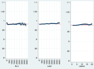
Figure 4 shows the partial effect of the control variables. The CONEAT index variable is statistically significant (p-value < 0.1%), and, when considering the other variables, a 10-point increase in the CONEAT index is expected to result in a 1% increase in meat production. Ranches without improvements over natural fields produce, on average, 3.2% less meat compared to those with improvements. Additionally, for each 1% expansion in the area of improved land, a corresponding 0.2% growth in meat production is expected (p-value < 0.1%). When examining livestock composition, ranches specialized in cattle farming exhibit 5.6% higher production compared to mixed ranches (p-value < 0.1%). Meanwhile, ranches oriented towards cow-calf production do not present significant differences when compared to those following a complete cycle of livestock farming (p-value = 0.384). Infrastructure-wise, we observe significant variations: producers equipped with livestock scales and cattle handling facilities yield 7.2% and 4.4% more meat production, respectively (p-value < 0.1% and p-value = 0.035), while factors such as the absence of electricity (p-value = 0.340), vehicle presence (p-value = 0.306), and the existence of a rainwater tank (p-value = 0.934) or a stock pond (p-value = 0.326) do not yield statistically significant differences.
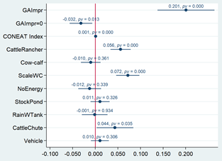
Figure 4: The 95% confidence intervals for partial effect of the control variables in the production function
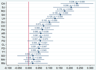
Lastly, geographical variations also impact production. Beef output in Canelones region exceeds that in Rivera (omitted category) by 23.6% after accounting for input usage and other variables (Figure 5). These discrepancies point to structural variations among different production regions not captured by the inputs and control variables in the model. In future research, it may be beneficial to explore the possibility of modeling spatial production variations by employing precise georeferencing data for each property, thereby achieving a better control over spatially unobservable heterogeneity.
3.2 Technical efficiency
When computing technical efficiency, we analyze the data in two distinct ways: weighting it by the size of the ranches in livestock units and treating all farms with equal weight (as shown in Figure 6). These two approaches yield two different indicators: the simple average efficiency of the farms in our sample, which is relevant for assessing the heterogeneity within our dataset, and a weighted average that provides a more representative measure of the state of the livestock sector in Uruguay.
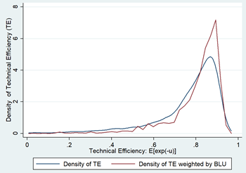
When using the weighted sample by size, it is observed that the average TE level increases from 76.2% to 79.1%, and the dispersion narrows (Table 2). This is evident as the p90/p10 ratio decreases from 59.2% to 41.2%.
Table 2: Descriptive statistics of the TE distribution estimated by the model
| 240. | Mean | 241.SD | 242.CV | 243.p10 | 244.p25 | 245.p50 | 246.p75 | 247.p90 | 248.p90/p10 |
|---|---|---|---|---|---|---|---|---|---|
| TE | 251.0.762 | 252.0.152 | 253.0.200 | 254.0.562 | 255.0.715 | 256.0.808 | 257.0.864 | 258.0.895 | 259.1.592 |
| TE* | 262.0.791 | 263.0.124 | 264.0.156 | 265.0.633 | 266.0.757 | 267.0.829 | 268.0.870 | 269.0.894 | 270.1.412 |
Note: TE is the simple average and TE* is the weighted average by livestock bovine units (BLU).
Table 3 presents the Pearson bivariate correlation coefficients between the estimated TE and the variables included in the model. TE shows a positive correlation with the output and all inputs, which may be influenced by the farm's size (we will come back to this point later).
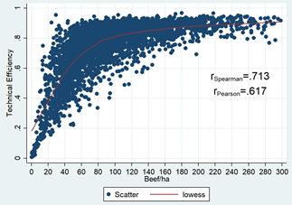
Figure 7 illustrates the relationship between TE and meat production per hectare, which is the standard performance measure for ranches. We have plotted a local regression between these two variables, revealing a nonlinear positive relationship. The Pearson correlation coefficient between the variables at the level is 0.6174, and in ranks (Spearman) it is 0.713. Notably, there seems to be a cutoff point at 80 kg/ha; for values lower than this, the Pearson correlation is 0.7364, whereas for values greater than 80 kg/ha, it drops to 0.3779.
Table 3: Pearson's correlation
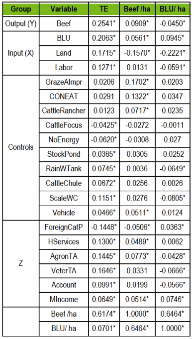
Note: values with * are statistically significant at 1%. Output and inputs are presented in level form to facilitate the interpretation.
To assess the influence of the explanatory variables on efficiency, we compute the average partial effect of each variable on the expected value and variance of technical inefficiency (as shown in Table 4). Standard errors are estimated using bootstrapping with 1000 iterations, following the methodology outlined by Kumbhakar and others27.
Table 4: Average partial effect (APE) of explanatory variables on expectation and variance of inefficiency
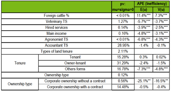
Note: standard errors of APE on E(u) and V(u) estimated by bootstrap with 1000 repetitions (*** pv<0.01; **pv<0.05: * pv<0.1). Categorical variable tenure and ownership type have as omitted category owner and individual ownership, respectively.
The variables that significantly affect the expected value of TE at the 1% level are: the ratio of foreign cattle (11.4%), possession of technical agronomic assistance (-6.8%), veterinary services (-5.7%), the main income sourced from the farm (-4.8%), and contracted services to external parties (-3.9%). Conversely, factors such as the ratio of foreign cattle (7.3%), the presence of technical agronomic assistance (-4.3%) and veterinary services (-3.7%), primary income being farm-related (-3.1%), and third-party hired services (-2.5%) are significantly related to the variance of the TE score. The variable accounting for technical assistance is not statistically significant at the 10% level.
This implies that, for example, ranches with agronomic technical assistance have an average level of technical inefficiency that is 6.8% lower than those without agronomic advice. Additionally, the variance of technical inefficiency for ranches with agronomic assistance is 4.3% lower than for those without such assistance.
When analyzing the data based on the types of land tenure, which include tenant, tenant-owner, and other forms (with the 100% owner category as the reference), we observe statistically significant lower levels (-7.3%) and variance (-4.8%) of inefficiency in other forms of tenure. This category encompasses various arrangements such as grazing for 11 months exclusively, sharecropping, occupants, and other similar forms.
Finally, when exploring the impact of the type of ownership, which includes corporate ownership with and without contracts (with individual ownership as the reference category), we discovered that farms owned by corporate ownership tend to have lower efficiency levels. Specifically, corporate ownership without contracts or successions exhibit a level and variance of technical inefficiency that are 25% and 16.5% lower than those owned by natural persons.
3.3 Descriptive analysis by TE deciles
As part of our exploratory analysis, we categorized ranches into ten equal-sized groups (deciles) based on their technical efficiency (TE), sorting them from lowest to highest TE. This categorization allowed us to describe the composition of these groups (Table 5, 6, 7 and 8). It is worth noting that given the multiple hypothesis tests conducted, we applied a Bonferroni correction38. The correction involves dividing the significance level (5%) by the number of comparisons, which in this case is 45 (representing combinations of 2 out of 10 groups). This correction helps to control for the increased risk of making a Type I error due to multiple testing.
An increasing relationship between TE and meat production per hectare is observed, corroborating the results commented above. However, it is important to note that not all the groups show statistically significant differences.
There is a positive association between TE and the size of the farm (measured in livestock units or grazing area), but there is no clear relationship between TE and the CONEAT index or the level of soil intensification.
Concerning the sheep-to-cattle ratio and the proportion of foreign-owned animals within the ranches, they are negatively associated with TE. In contrast, TE shows a positive association with the availability of technical advice (including agronomic, veterinary, or accounting assistance), infrastructure resources, and access to hired services. Additionally, the relationship between the ratio of bovine livestock units (BLU) per hectare and TE follows an inverted U-shaped pattern.
Remarkably, the decile associated with the lowest TE also exhibits a cattle mortality rate of 6.4%, which is over twice the overall average of 2.6%.
Table 5: Descriptive statistics by decile of technical efficiency (TE)
| TE decile | 309.TE | 310.Beef/Land | 311.BLU | 312.GrAr Improved | 313.Land | 314.CONEAT | 315.Land/Labour |
|---|---|---|---|---|---|---|---|
| 1 | 318.0.396 | 319.37 | 320.277 C | 321.0.115 AB | 322.381 B | 323.86 A | 324.178 C |
| 2 | 327.0.63 | 328.62 | 329.397 A C | 330.0.111 A | 331.495 AB | 332.84 A | 333.231 AB |
| 3 | 336.0.715 | 337.76 | 338.425 ABC | 339.0.106 A | 340.508 AB | 341.88 A | 342.216 A C |
| 4 | 345.0.762 | 346.86 A | 347.417 ABC | 348.0.113 A | 349.524 AB | 350.86 A | 351.226 ABC |
| 5 | 354.0.794 | 355.92 AB | 356.536 AB D | 357.0.105 A | 358.648 A C | 359.86 A | 360.244 AB |
| 6 | 363.0.82 | 364.98 BC | 365.538 AB D | 366.0.092 A | 367.681 A CD | 368.86 A | 369.246 AB |
| 7 | 372.0.843 | 373.104 C | 374.554 B DE | 375.0.096 A | 376.684 A CD | 377.86 A | 378.253 AB |
| 8 | 381.0.864 | 382.114 | 383.692 E | 384.0.117 AB | 385.860 D | 386.88 A | 387.263 AB |
| 9 | 390.0.884 | 391.125 | 392.655 DE | 393.0.12 AB | 394.821 CD | 395.88 A | 396.267 B |
| 10 | 399.0.913 | 400.154 | 401.482 AB | 402.0.156 B | 403.615 A | 404.90 A | 405.225 ABC |
| Total | 408.0.762 | 409.95 | 410.497 | 411.0.113 | 412.622 | 413.87 | 414.235 |
Note: groups with the same letter do not present statistically significant differences (𝛼=5%/𝑚=1/900=0.1%).
Table 6: Descriptive statistics by decile of technical efficiency (TE)
| TE decile | 421.TE | 422.BLU/Land | 423.Ovine LU*5/BLU | 424.% Foreign Owned Cattle | 425.Agronomic TA | 426.Veterinary TA | 427.Accountant TA |
|---|---|---|---|---|---|---|---|
| 1 | 430.0.396 | 431.0.783 C | 432.0.761 A | 433.0.192 B | 434.0.162 A | 435.0.298 D | 436.0.093 A |
| 2 | 439.0.63 | 440.0.845 ABC | 441.0.676 A | 442.0.178 B | 443.0.174 AB | 444.0.332 DE | 445.0.077 A |
| 3 | 448.0.715 | 449.0.884 AB | 450.0.673 A | 451.0.123 A | 452.0.2 ABC | 453.0.358 B DE | 454.0.087 A |
| 4 | 457.0.762 | 458.0.902 A | 459.0.724 A | 460.0.123 A | 461.0.206 ABC | 462.0.409 B E | 463.0.109 A |
| 5 | 466.0.794 | 467.0.899 A | 468.0.743 A | 469.0.106 A | 470.0.217 ABC | 471.0.455 AB | 472.0.138 ABC |
| 6 | 475.0.82 | 476.0.891 A | 477.0.735 A | 478.0.119 A | 479.0.253 BCD | 480.0.447 AB | 481.0.119 A |
| 7 | 484.0.843 | 485.0.884 AB | 486.0.7 A | 487.0.103 A | 488.0.269 CD | 489.0.514 A C | 490.0.128 A C |
| 8 | 493.0.864 | 494.0.892 A | 495.0.734 A | 496.0.084 A | 497.0.328 DE | 498.0.538 A C | 499.0.192 BC |
| 9 | 502.0.884 | 503.0.876 AB | 504.0.661 A | 505.0.095 A | 506.0.358 E | 507.0.545 A C | 508.0.204 B |
| 10 | 511.0.913 | 512.0.813 BC | 513.0.679 A | 514.0.086 A | 515.0.449 BC | 516.0.593 C | 517.0.206 B |
| Total | 520.0.762 | 521.0.867 | 522.0.709 | 523.0.121 | 524.0.261 | 525.0.449 | 526.0.135 |
Note: groups with the same letter do not present statistically significant differences (𝛼=5%/𝑚=1/900=0.1%).
Table 7: Descriptive statistics by decile of technical efficiency (TE)
| TE decile | 533.TE | 534.M Income | 535.H Services | 536.Scale WC | 537.Stock Pond | 538.Cattle Chute | 539.Rainwater Tank |
|---|---|---|---|---|---|---|---|
| 1 | 542.0.396 | 543.0.822 A | 544.0.601 C | 545.0.136 D | 546.0.593 A | 547.0.879 B | 548.0.117 AB |
| 2 | 551.0.63 | 552.0.85 AB | 553.0.668 BC | 554.0.178 CD | 555.0.63 A | 556.0.915 AB | 557.0.115 B |
| 3 | 560.0.715 | 561.0.872 AB | 562.0.676 BC | 563.0.235 ABC | 564.0.626 A | 565.0.917 AB | 566.0.13 AB |
| 4 | 569.0.762 | 570.0.87 AB | 571.0.749 AB | 572.0.221 A CD | 573.0.603 A | 574.0.931 AB | 575.0.15 ABC |
| 5 | 578.0.794 | 579.0.883 AB | 580.0.767 A | 581.0.255 ABC | 582.0.611 A | 583.0.957 A | 584.0.182 ABC |
| 6 | 587.0.82 | 588.0.883 AB | 589.0.747 AB | 590.0.239 ABC | 591.0.658 A | 592.0.947 A | 593.0.18 ABC |
| 7 | 596.0.843 | 597.0.879 AB | 598.0.753 AB | 599.0.279 AB | 600.0.621 A | 601.0.945 A | 602.0.192 A C |
| 8 | 605.0.864 | 606.0.879 AB | 607.0.796 A | 608.0.312 B | 609.0.678 A | 610.0.947 A | 611.0.223 C |
| 9 | 614.0.884 | 615.0.915 B | 616.0.787 A | 617.0.296 AB | 618.0.658 A | 619.0.929 AB | 620.0.19 ABC |
| 10 | 623.0.913 | 624.0.885 AB | 625.0.812 A | 626.0.283 AB | 627.0.68 A | 628.0.931 AB | 629.0.192 A C |
| Total | 632.0.762 | 633.0.874 | 634.0.736 | 635.0.243 | 636.0.636 | 637.0.93 | 638.0.167 |
Note: groups with the same letter do not present statistically significant differences (𝛼=5%/𝑚=1/900=0.1%).
Table 8: Descriptive statistics by decile of technical efficiency (TE)
| TE decile | 645.TE | 646.Mortality/Stock | 647.Individual ownership | 648.Corporate ownership | 649.Paddocks |
|---|---|---|---|---|---|
| 1 | 652.0.396 | 653.0.063 | 654.0.081 A | 655.0.84 B | 656.6.1 E |
| 2 | 659.0.63 | 660.0.033 D | 661.0.081 A | 662.0.83 AB | 663.7.5 B E |
| 3 | 666.0.715 | 667.0.027 CD | 668.0.101 AB | 669.0.81 AB | 670.8.7 AB |
| 4 | 673.0.762 | 674.0.025 BC | 675.0.109 AB | 676.0.81 AB | 677.8.3 AB |
| 5 | 680.0.794 | 681.0.02 ABC | 682.0.119 AB | 683.0.81 AB | 684.9.1 ABC |
| 6 | 687.0.82 | 688.0.02 AB | 689.0.111 AB | 690.0.82 AB | 691.9.4 A C |
| 7 | 694.0.843 | 695.0.018 AB | 696.0.128 AB | 697.0.82 AB | 698.9.4 A C |
| 8 | 701.0.864 | 702.0.018 A | 703.0.15 B | 704.0.78 AB | 705.11.5 D |
| 9 | 708.0.884 | 709.0.019 AB | 710.0.166 B | 711.0.75 A | 712.11.5 D |
| 10 | 715.0.913 | 716.0.023 ABC | 717.0.144 AB | 718.0.77 AB | 719.10.8 CD |
| Total | 722.0.762 | 723.0.026 | 724.0.119 | 725.0.8 | 726.9.2 |
Note: groups with the same letter do not present statistically significant differences (??=5%/𝑚=1/900=0.1%).
3.4 Descriptive analysis using regression trees
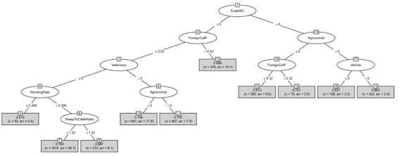
Figure 8 depicts the regression tree, dividing livestock ranches based on the average TE. The tree effectively segments ranches into 10 end nodes, reflecting the heterogeneity of the results, with average technical efficiency groups spanning from 61% to 86.5%.
The algorithm starts the segmentation process by assessing whether there is a cattle weighing scale present. The presence of such a scale suggests more precise herd management, indicating better overall farm management or TE.
Lower levels of TE are found in groups that lack technical assistance, and are distinguished by either a low ratio of livestock units to surface area (below 0.368) or a high percentage of third-party-owned livestock (above 53%). The presence of agronomic and veterinary technical advisory services divides the farms, with higher levels of efficiency observed in those ranches that utilize these services.
3.5 Robustness test
Finally, to ensure the reliability and robustness of our results, we conducted some additional tests. Initially, we ran the model while excluding outliers. Among the 5,057 farms included in our analysis, only eleven were identified as outliers. While we have not presented the specific results in this section, it is important to note that the outcomes of these tests were consistent with the main findings we have discussed earlier in the study.
As part of our robustness checks, we conducted a second test. In this test, we adjusted the inconsistency filter related to the information reported in stock versus recorded cattle movements. The greater the level of inconsistency, the less credible the data become, and this, by definition, affects the estimated value of meat production9. Initially, we used a tolerance range of -5% to 5% for discrepancies, but in this test we have expanded the range to -25% to 25% of the herd. This relaxation of the filter criteria resulted in an increase in the number of farms meeting the filters, growing from the initial 5,057 to more than 8,075 ranches.
It is important to note that even with this adjustment, the results remained qualitatively consistent across various aspects, including input-output elasticities, returns to scale, and the influence of explanatory variables on efficiency. However, the notable change was a decrease in the average efficiency rate, which dropped to 70.9%. This makes sense, especially considering that we are adding more than 3,000 ranches.
4. Discussion
In a context where projections anticipate ongoing growth in global beef demand, increasing livestock productivity represents a significant opportunity for rural development in Uruguay. This enhancement is essential for stimulating economic development, boosting the competitiveness of cattle farms, and ensuring food security. Moreover, enhancing livestock productivity is crucial for meeting the goals associated with sovereign bonds indexed to environmental sustainability indicators23.
Through this study, our objective is to contribute to the expanding field of research concerning TE in beef cattle farming. We specifically concentrate on one of the three primary avenues for enhancing productivity over time, which is TE. The other two pathways involve technological advancements and productivity improvements resulting from changes in scale. Gaining a thorough understanding of these efficiency aspects is of utmost importance, as it can provide essential guidance for the development, targeting, monitoring, and assessment of evidence-based policy measures.
In this paper, we present novel estimates of the production function and TE in Uruguayan beef cattle farming. Our analysis is based on comprehensive data derived from the national census and administrative records for individual farms across the country. We find that the average TE stands at 76.2%. This result is consistent with previous studies conducted in Uruguay, such as García-Suárez, Pérez-Quesada, and Molina21, who reported an efficiency level of 76.9%, and García-Suárez and Lanfranco20, who found a TE of 72.3%.
The overall average TE masks significant variations, as the most efficient farm in the top decile achieves 89.5% efficiency, which stands in stark contrast to the bottom 10% with only 56.2% efficiency. This substantial difference results in a remarkable 59.2% increase in efficiency when moving from the lowest to the highest decile (by TE).
When we account for farm size by weighting the data for bovine livestock units (BLU), the TE average increases to 79.1%, compared to an unadjusted mean of 76.2%. This adjustment highlights the frequent lower efficiency found in smaller farms. With this 79.1% efficiency level, there is the potential to produce an additional 26% of beef using the existing resources and technology, implying a significant opportunity for productivity improvement.
Our analysis of TE disparities aligns with previous Uruguayan researches, which also emphasized significant production variations across farms based on administrative records 8)(10)39)(40) . However, our findings indicate a reduction in these variations, likely attributed to the consideration of heterogeneity in inputs, infrastructure, technology, and advisory services.
The input-output elasticities and returns to scale exhibit positive values consistent with theoretical expectations. However, these values vary across ranches. Farms with fewer than 400 BLU show a more pronounced response in meat production to changes in animal allocation. Additionally, our findings suggest that returns to scale may not be constant, particularly exceeding the mean value for farms with fewer than 100 BLU.
Indeed, given the significance of fixed costs in influencing economies of scale, it would be valuable for future research to compute scale elasticity while considering a stochastic net income function. Furthermore, delving into economic modeling of ranch decisions that incorporates factors like opportunity costs and risks could be a pertinent direction for upcoming studies.
Interpreting the results of our study requires caution due to the cross-sectional nature of the data and the assumption of input exogeneity. In the TE literature, there are two approaches to endogenize input use: using a statistical model with instrumental variables or employing an economic model based on a structural framework26. Nevertheless, in our case involving cross-sectional census data, the task of identifying appropriate instrumental variables or accurately specifying the objective function which producers would intend to optimize remains a challenging endeavor.
Shifting our attention to another critical aspect, climate plays a significant role in beef cattle farming, particularly in pasture growth. Uruguay benefits from low-altitude relief, a temperate climate, and evenly distributed rainfall throughout the year, although there are notable annual variations. However, quantifying the influence of climate through specific variables can be challenging. In our technical efficiency model, we typically controlled the farm's geographical region. Future research could enhance this analysis by georeferencing farms and utilizing satellite imagery to more accurately assess conditions such as soil moisture, forage quality, and production levels.
Another limitation of our study is the reliance on data from a single snapshot in time, considering the inherent inertia of beef farming due to long-term biological cycles. The development of dynamic models for beef production represents an important avenue for future research. This challenge is further complicated by the frequency of available data, as the response of variables is likely to vary across different time periods or windows. Furthermore, having access to panel data would allow the use of less restrictive models and improved control for unobservable heterogeneity, providing a more nuanced understanding of the factors influencing production efficiency.
As expected, variables related to improved animal management practices, such as weighing scales, cattle chutes, and technological guidance, exhibit a positive correlation with efficiency. While causality remains uncertain, this association highlights a meaningful connection between technical advice and efficiency, even after accounting for input levels, regional differences, and technology.
Finally, evaluating technical efficiency at the individual livestock farm level provides a deeper understanding of farm management practices. This fine-grained perspective facilitates direct comparisons among diverse production units, thereby yielding more precise insights into the efficacy of livestock-related programs and policies. This granularity is especially pertinent since technical efficiency serves as a superior outcome variable for evaluating the effects of interventions on the livestock population, offering a more targeted and meaningful measure for evaluating success and identifying areas for improvement.