


Serviços Personalizados
Journal

Artigo
 Inglês (pdf)
 Artigo em XML
 Referências do artigo
Links relacionados
Compartilhar

 Permalink
CLEI Electronic Journal
versão On-line ISSN 0717-5000
CLEIej vol.17 no.1 Montevideo abr. 2014
Abstract
Cooperative coevolutionary evolutionary algorithms differ from standard evolutionary algorithms’ architecture in that the population is split into subpopulations, each of them optimising only a sub-vector of the global solution vector. All subpopulations cooperate by broadcasting their local partial solutions such that each subpopulation can evaluate complete solutions. Cooperative coevolution has recently been used in evolutionary multi-objective optimisation, but few works have exploited its parallelisation capabilities or tackled real-world problems. This article proposes to apply for the first time a state-of-the-art parallel asynchronous cooperative coevolutionary variant of the non-dominated sorting genetic algorithm II (NSGA-II), named CCNSGA-II, on the injection network problem in vehicular ad hoc networks (VANETs). This multi-objective optimisation problem, consists in finding the minimal set of nodes with backend connectivity, referred to as injection points, to constitute a fully connected overlay that will optimise the small-world properties of the resulting network. Recently, the well-known NSGA-II algorithm was used to tackle this problem on realistic instances in the city-centre of Luxembourg. In this work we analyse the performance of the CCNSGA-II when using different numbers of subpopulations, and compare them to the original NSGA-II in terms of both quality of the obtained Pareto front approximations and execution time speedup.
Resumen
Los algoritmos evolutivos cooperativos coevolutivos difieren de la arquitectura de los algoritmos evolutivos estándares en que la población se divide en sub-poblaciones, cada una de ellas dedicada a la optimización de un único sub-vector del vector que forma la solución global al problema. Todas las sub-poblaciones cooperan haciendo pública su mejor solución parcial local, de forma que cada subpoblación pueda evaluar soluciones completas usando esta información. La coevolución cooperativa se ha utilizado recientemente en algoritmos evolutivos de optimización multi-objetivo, pero muy pocos trabajos han explotado su capacidad de paralelismo o se han enfocado a problemas del mundo real. Este artículo propone aplicar, por primera vez, un algoritmo evolutivo cooperativo coevolutivo paralelo y asíncrono, variante del algoritmo NSGA-II, y llamado CCNSGA-II, para el problema de la inyección de enlaces en redes ad hoc vehiculares (VANETs). Este problema de optimización multi-objetivo consiste en encontrar el conjunto mínimo de nodos con conectividad adicional, llamados puntos de inyección, para formar una red subyacente completamente conectada de forma que las características de mundo pequeño de la red resultante sean optimizadas. Recientemente, el conocido algoritmo NSGA-II se utilizó para resolver este problema en instancias realistas del centro de la ciudad de Luxemburgo. En este trabajo analizamos el rendimiento de CCNSGA-II con distintos números de sub-poblaciones, y lo comparamos con el NSGA-II original en función de la calidad de la aproximación al frente de Pareto obtenido y del tiempo de ejecución.
Keywords: Multi-objective optimisation, VANETs, small-world, topology control.
Spanish keywords: optimización multi-objetivo, mundos pequeños, control de topología.
Received: 2013-09-08; Revised: 2013-03-01 ; Accepted: 2013-03-10
Real-world optimisation problems are typically hard and multi-objective by nature, since different conflicting criteria have to be considered. This means that in such problems improving one objective will imply decreasing (some of) the others. Contrary to single-objective optimisation which aims to a unique solution, multi-objective optimisation consists in finding a set of so-called non-dominated solutions in the objective space, referred to as Pareto-front. A solution is said to dominate another one if it is better on one objective and similar or better on the other objectives. A multi-objective algorithm then aims to find a limited set of non-dominated solutions as close as possible to the optimal Pareto-front, both in terms of diversity and convergence.
Since many years, Evolutionary algorithms (EAs) have proven to be an efficient approach for multi-objective optimisation [ 1]. However standard multi-objective EAs have shown some limits when dealing with large and complex problems, which motivated research in faster and more accurate methods. One promising approach is cooperative coevolution as introduced originally by Potter for single-objective optimisation [ 2], in which the solution vector is decomposed and each subset of solution is evolved in a separated subpopulation. These cooperate by exchanging their local representative(s) in order to create a complete solution to be evaluated on the global problem.
Some recent works have also demonstrated the advantages of cooperative coevolution in the multi-objective context [ 3, 4], most of them focused on improving the solutions quality. As originally stated by Potter, cooperative coevolution has some good potential for parallelism, but only few works have studied this capability. Most lately, Nielsen et al. proposed a new parallel asynchronous cooperative coevolutionary non-dominated sorting genetic algorithm II (CCNSGA-II) [ 5] that demonstrated promising speedup capabilities but limited their study to well-known multi-objective benchmark functions.
In this work we thus propose to apply for the first time this state-of-the-art algorithm on a real-world problem, i.e., the injection network problem in vehicular ad hoc networks (VANETs). This topology control problem consists in finding the minimum set of vehicles, called injections points, chosen to provide backend connectivity and compose a fully-connected overlay network such that small-world properties of the resulting network are optimised. Additionally, we study the impact of the number of subpopulations used on the performance of the algorithm. Experiments are conducted on realistic VANET networks snapshots from Luxembourg city, generated with the VehILux mobility model [ 6]. This paper is an extension of our previous work [ 7].
The remainder of this article is organised as follows. The next section presents a brief state-of-the-art on cooperative coevolutionary multi-objective EAs. Then the NSGA-II algorithm and its asynchronous cooperative coevolutionary variant (CCNSGA-II) are presented in detail in section 3. The injection network problem is described in section 4. Section 5 then provides the experimental setup and results analysis in terms of execution time speedup and solution quality. Finally our conclusions and perspectives and given in section 6.
Cooperative coevolutionary evolutionary algorithms (CCEAs) mainly differ from standard EAs by their fitness evaluation that requires interactions with individuals from other so-called subpopulations. In the original cooperative coevolution framework proposed by Potter et al. in [ 2], the decision vector is split such that each decision variable is evolved in different subpopulations. In order to evaluate their partial solutions, each subpopulation exchanges periodically some representative (e.g. best) with all other subpopulations. This coevolutionary framework was initially proposed for single-objective optimisation but more recently several multi-objective versions proved to be efficient [ 1]. The following proposes a brief survey of cooperative coevolutionary MOEAs, a more comprehensive one can be found in [ 8].
The first CCMOEA was proposed in [ 9] as an extension of the Genetic Symbiosis Algorithm (GSA) for multi-objective optimisation problems. The multi-objective GSA (MOGSA) differs from the standard GSA with a second symbiotic parameter, which represents the interactions of the objective functions. One main drawback of this algorithm is that it requires knowledge of the search space, which highly reduces its application possibilities.
Then, Keerativuttitumrong et al. proposed the Multi-objective Co-operative Co-evolutionary Genetic Algorithm (MOCCGA) in [ 10]. It combines Fonseca and FlemingÕs multi-objective GA (MOGA) and Potter’s Co-operative Co-evolutionary Genetic Algorithm (CCGA). Each subpopulation evolves using MOGA and assigns a fitness to its individuals based on their rank in the subpopulation local Pareto front. However this local Pareto optimality perception is a limiting factor for the performance of MOCCGA. A parallel implementation of MOCCGA was empirically validated using 1, 2, 4 and 8 cores, but limited to well-known benchmark functions (ZDT [ 11]).
MOCCGA was extended in [ 12], with other MOEAs and a fixed size archive that stores the non-dominated solutions. Another variant was introduced by Tan et al. [ 4] proposed, in addition to adding an archive, a novel adaptive niching mechanism. A parallel version was also experimented but still limited to the ZDT benchmark. Finally, [ 3] presented a non-dominated sorting cooperative coevolutionary algorithm (NSCCGA), which is essentially the coevolutionary extension of NSGA-II.
Most lately, Dorronsoro et al. proposed a parallel synchronous CCMOEA framework with three different MOEAs [ 8]: NSGA-II, Strength Pareto Evolutionary Algorithm (SPEA2) [ 13] and Multi-objective Cellular Genetic Algorithm (MOCell) [ 14]. They demonstrated that super-linear speedup is possible on a scheduling problem, compared to the original MOEAs. Finally, a new variant with asynchronous communications between the subpopulations was proposed in [ 5] which further improved the speedup without degrading the solutions quality on standard benchmarks (i.e., DTLZ [ 15] and ZDT).
This article proposes to apply for the first time this parallel asynchronous CCMOEA with NSGA-II on a real-world problem, i.e., the optimisation of small-world properties in VANETs.
The following subsections present the two multi-objective algorithms considered in this work, the well-known Non-dominated Sorting Genetic Algorithm II (NSGA-II) and its cooperative coevolutionary variant CCNSGA-II.
3.1 Non-dominated Sorting Genetic Algorithm (NSGA-II)
The NSGA-II [ 16] algorithm is the reference algorithm in multi-objective optimisation. A pseudocode is given in Algorithm 1. NSGA-II does not implement an external archive of non-dominated solutions, but the population itself keeps the best non-dominated solutions found so far. The algorithm starts by generating an initial random population and evaluating it (lines 2 and 3). Then, it enters in the main loop to evolve the population. It starts by generating a second population of the same size as the main one. It is built by iteratively selecting two parents (line 6) by binary tournament based on dominance and crowding distance (in the case the two selected solutions are non-dominated), recombining them (two-point crossover in our case) to generate two new solutions (line 7), which are mutated in line 8 (here bit flip mutation) and added to the offspring population (line 9). The number of times this cycle (lines 5 to 10) is repeated is the population size divided by two, thus generating the new population with the same size as the main one. This new population is then evaluated (line 11), and merged with the main population (line 12). Now, the algorithm must discard half of the solutions from the merged population to generate the population for the next generation. This is done by selecting the best solutions according to ranking and crowding, in that order. Concretely, ranking consists on ordering solutions according to the dominance level into different fronts (line 13). The first front is composed by the non-dominated solutions in the merged population. Then, these solutions in the first front are removed from the merged population, and the non-dominated ones of the remaining solutions compose the second front. The algorithm iterates like this until all solutions are classified. To build the new population for the next generation, the algorithm adds those solutions in the first fronts until the population is full or adding a front would suppose exceeding the population size (line 14). In the latter case (lines 15 to 17), the best solutions from the latter front according to crowding distance (i.e., those solutions that are more isolated in the front) are selected to complete the population. The process is repeated until the termination condition is met (lines 4 to 18).
2: InitialisePopulation(nsga.pop);
3: EvaluatePopulation(nsga.pop);
4: while ! StopCondition() do
5: for index
 to nsga.popsize/2 do
 6:
 parents
 SelectParents(nsga.pop);
 7:
 children
 Crossover(nsga.Pc,parents);
 8:
 children
 Mutate(nsga.Pm,children);
 9:
 nsga.pop’
 Add(children);
 10: end for
11: EvaluatePopulation(nsga.pop’);
12:
 union
union Merge(nsga.pop, nsga.pop’);
 13:
 fronts
 SortFronts(union);
 14:
 (nsga.pop’, lastFront)
 GetBestCompleteFronts(fronts);
 15: if size(nsga.pop’)
 nsga.popsize then
 16:
 nsga.pop’
 BestAccToCrowding(lastFront,nsga.popsize-size(nsga.pop’));
 17: end if
18: end while
3.2 Asynchronous Cooperative Coevolutionary NSGA-II
As previously mentioned, cooperative coevolution splits the solution vector and evolves each subset of the solution using a genetic algorithm, in our case NSGA-II, in so-called subpopulations. In the single-objective case, each subpopulation then broadcasts its representatives to all the other subpopulations after each generations following a selection scheme (e.g., best individual). This fully connected broadcast of representatives enables each subpopulation to assemble and evaluate the resulting global objective function which is essential for the local genetic algorithm.
To apply the coevolutionary paradigm in the multi-objective context, several changes to the single-objective framework must be operated. The CCNSGA-II is based on the asynchronous cooperative coevolutionary framework which pseudo-code is given in Algorithm 2 and described in the following. A first difference is the merge of the local Pareto-front from each sub-population to generate an archive of best combined Pareto-fronts, as can be seen in line 16. This merging process of the solutions sets is done by choosing one of the sets and adding to it all the other solutions. If the resulting approximation set exceeds the archive size, the crowding policy is used to remove solutions based on the distance to surrounding individuals belonging to the same rank.
2: {
 means parallel run}
 3:
![Ⅎ i ∈ [1,I] ::](/img/revistas/cleiej/v17n1/1a0219x.png) InitialisePopulation(
InitialisePopulation( ,
,  ) {Initialise every subpopulation}
 4: Sync() {Synchronisation point}
5: {
 means sequential run}
 6:
![∀ i ∈ [1,I] ::](/img/revistas/cleiej/v17n1/1a0223x.png) BroadcastRepresentatives(
BroadcastRepresentatives( ,
,  ) {Send random local partial solutions to all subpopulations}
 7:
![Ⅎ i ∈ [1,I] ::](/img/revistas/cleiej/v17n1/1a0226x.png) EvaluatePopulation(
EvaluatePopulation( ,
,  ) {Evaluate solutions in every subpopulation}
 8: Sync()
9:
![Ⅎ i ∈ [1,I] ::](/img/revistas/cleiej/v17n1/1a0229x.png) {
{ 10: while ! StopCondition( ) do
11: generation(
 ,
,  ) {Perform one generation to evolve the population}
 12: broadcast(
 ,
,  ) {Share best local partial solutions in every subpopulation}
 13: end while
}
14: mergeParetoFronts( ) {Merge all subpopulations Pareto fronts into a single one}
A second difference induced by the multi-objective design lies in the construction of complete solutions for evaluation. As previously mentioned, in the single-objective case a partial solution from one subpopluation is evaluated by composing a complete solution with the best partial solutions received from all the other subpopulations. Whereas, in the multi-objective case, there will be most of the time more than a single best solution, i.e., a set of non-dominated solutions. In the CCNSGA-II, every subpopulation shares a number  of solutions randomly chosen from the non-dominated ones found so far. An example of how one sub-population,
  , shares four of its best solutions (i.e.,
  ) with the other two populations is presented in Fig. 1. In case the local Pareto-front contains less than
  non-dominated solutions, randomly chosen individuals are taken from the rest of the population to complete the set of
  solutions.
In this asynchronous variant, contrary to the original synchronous model, there is no synchronisation point before the broadcasting of the solutions (i.e., synchronisation would be inserted in line 12). Subpopulations keep evolving independently even when the other subpopulations are still busy with the current generation. This means that the subpopulations will not share the total number of available objective function evaluations equally between them. A fast executing subpopulation might perform more evaluations and thus ’steal’ evaluations from the slower subpopulations. Even if all subpopulations do ’consume’ the same amount of total function evaluations, the asynchronous version should remove delays and allow the algorithm to finish faster. Another possible consequence of the asynchronicity is that a subpopulation may start evaluating its individuals before the other subpopulations have transmitted their own individuals, i.e., old individuals are used. However this effect was shown to have no statistical significant impact on the results quality compared to the synchronous model [ 5].
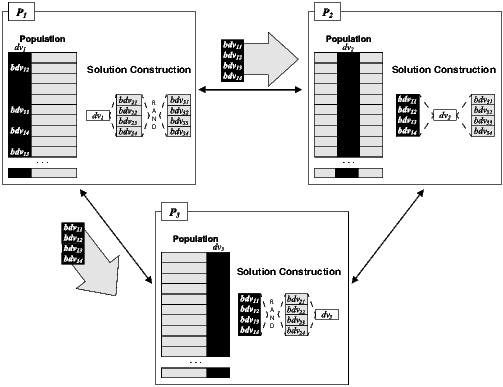
 ) shares with the other coevolving populations (
 and
and  ) its four best partial solutions (
 to
to  ). The partial solutions are evaluated by building complete solutions with random partial solutions of the other two subpopulations (
 and
and  )
)
The injection network problem considered in this work was originally introduced in [ 17]. Provided a snapshot of a VANET, the objective is to determine the best set of vehicles to join the overlay network in order to unpartition the corresponding network graph and maximise its small-world properties. In the first subsection the injection network problem is defined together with the small-world metrics used. The second subsection defines the corresponding multi-objective optimisation problem.
This problem considers hybrid VANETs where each vehicle can potentially have both vehicle-to-vehicle and vehicle-to-infrastructure (e.g., using Wi-Fi hotspots) communications. Nodes elected as injection points (i.e., nodes connected to the infrastructure) form a fully connected overlay network, that aims at increasing the connectivity and robustness of the VANET. Injection points respectively permit to efficiently disseminate information from distant and potentially disconnected nodes and prevent costly bandwidth overuse with redundant information. An example network is presented in Figure 2.
In this problem, we consider small-world properties as indicators for the good set of rules to choose injection points. Small-World networks [ 18] are a class of graphs that combines the advantages of both regular and random networks with respectively a high clustering coefficient (CC) and a low average path length (APL). The APL is defined as the average of the shortest path length between any two nodes in a graph  , that is
 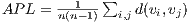 with
with  the shortest distance between nodes
  ,
,  . It thus indicates the degree of separation between the nodes in the graph. The local
  of node
  with
with  neighbours is
 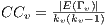 where
where  is the number of links in the relational neighbourhood of
  and
and  is the number of possible links in the relational neighbourhood of
  . The global clustering coefficient is the average of all local
  in the network, denoted as
 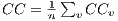 . The CC measures to which extent strongly interconnected groups of nodes exist in the network, i.e., groups with many edges connecting nodes belonging to the group, but very few edges leading out of the group.
We here consider Watts original definition of the small world phenomenon in networks with  and
and  , where
  and
and  are, respectively, the
  and
and  of random graphs with similar number of nodes and average node degree
  . In addition, the number of chosen injection points has to be minimised as they may induce additional communication costs.
The proposed optimisation problem can be formalised as follows. The solution to this problem is a binary vector  of size
  (number of nodes in the network),
 ![s[1..n]](/img/revistas/cleiej/v17n1/1a0272x.png) where
where ![s[i] = 1](/img/revistas/cleiej/v17n1/1a0273x.png) if node
if node  is an injection point, and
 ![s[i] = 0](/img/revistas/cleiej/v17n1/1a0275x.png) if
if  is not an injection point. The decision space is thus of size
  .
.
This problem is a three objectives one, defined as:
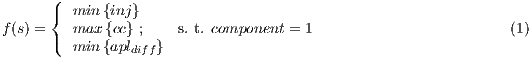
where  is the number of chosen injection points,
  is the average clustering coefficient of the resulting network, and
  is the absolute difference between the APL of the resulting network and the APL of the equivalent random graph:
 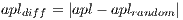 . For each overlay network instance evaluated in this work, the
  and
and  is obtained by averaging the
  and
and  of 30 corresponding random graphs using Watts random rewiring procedure with probability
  [ 18]. Each random graph is created based on the number of devices and average network degree. Since the initial objective is to unpartition the network, a constraint is set on the number of connected components in the created network, i.e.,
  must be equal to 1.
This section first describes the methodology we followed for our experiments, i.e., the algorithms and problem instances parameters. In the second subsection the obtained results considering both solutions quality and speedup are presented and analysed.
The configuration of the NSGAII algorithm used in the subpopulations is the same as for the ‘standard’ NSGAII, except the length of the decision vector. Indeed, for the NSGAII, the length is equal to the total number of nodes in the problem instance, whereas for the CCNSGAII it is divided by the number of subpopulations.
The parameters of the algorithms are presented in Table 1. The configuration of the NSGAII is the one originally suggested by the authors [ 16]. However, some parameters were adapted because a binary representation was used, in which each gene (i.e., bit) represents one car. Genes set to 1 mean that the corresponding cars act as injection points, while a 0 value indicates the contrary The two-point crossover operator (DPX) with probability  and the bit-flip mutation operator with probability
  were used. In two-point recombination, two crossover positions are selected uniformly at random in both parents, and the values between these points are exchanged to generate two new offspring solutions. The bit-flip mutation is to change a 1 into a 0, or vice-versa. The algorithm evolves until
  fitness function evaluations are performed, and 30 independent runs were executed for every problem instance.
The CCNSGAII uses 4, 8, and 12 subpopulations, each of them is run in a separate thread running on a different core of the same multi-processor machine. The population size for the NSGAII is 100, and every subpopulation also has 100 individuals in the studied CCNSGAII. Islands are exchanging 20 randomly chosen local non-dominated solutions, and to evaluate a given solution, it is built with random sub-solutions from those shared by the other subpopulations, as proposed in [ 8].
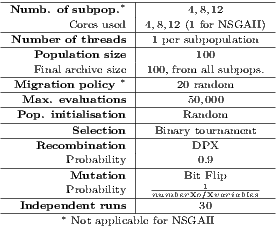
For the problem instances, we have used snapshots from realistic VANET scenarios in the city centre of Luxembourg, simulated using the VehILux mobility model [ 6]. VehILux accurately reproduces the vehicular mobility in Luxembourg by exploiting both realistic road network topology (OpenStreetMaps) and real traffic counting data from the Luxembourg Ministry of Transport. The 6 studied networks represent snapshots of a simulated area of 0.6  , the first three small snapshots are taken between 6:00 a.m. and 6:15 a.m. and the three large ones between 7:00 a.m. and 7:15 a.m. The properties of the instances are shown in Table 2.
This section presents the results obtained in our experiments. These were run on the HPC facility of the University of Luxembourg. The nodes used are HP Proliant BL2x220c G6 (10U) with 2 Intel L5640 CPU’s having 6 cores each at 2.26 GHz.
The first part focuses on the analysis of the speedup obtained and the second part analyses the solutions found by the algorithms according to the following two well-known quality measures (accounting for solutions diversity and convergence): unary additive epsilon ( ) and spread (
 ).
).

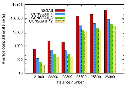
The first objective of this work is to study the benefit of the parallel asynchronous CCNSGAII in terms of computational time speedup and solutions quality with three different numbers of subpopulations, namely 4, 8 and 12, and compare them to the standard NSGAII. We call the algorithms CCNSGA_4, CCNSGA_8, and CCNSGA_12 according to the number of subpopulations used. All numerical results obtained for the execution time and speedup studies are given in Table 3.
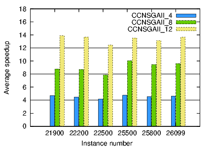
Figures 3 and 4 presents the average execution times in seconds for the six problem instances and the corresponding speedup factor, respectively. The execution times increase drastically together with the problems instance sizes, from 121.18 seconds for the fastest with CCNSGAII on the smallest instance (21900), to more than 107 hours with NSGAII on the largest instance (26099). This very large computational time justifies the search for efficient parallel optimisation approaches. We can see how increasing the number of islands leads to significantly shorter execution times for all problem instances (notice that time is in logarithmic scale in Fig. 3).
Regarding the speedup (shown in Fig. 4), we can see that all coevolutionary algorithms perform super-linear speedups for all problems, with respect to the original NSGAII algorithm. The only exception is CCNSGAII_8 for problem 22500, for which the speedup achieved is almost linear. The average speedup obtained is 4.55, 9.07, an 13.38 for CCNSGAII_4, CCNSGAII_8, and CCNSGAII_12, respectively. Therefore, we can see that there are super-linear speedups if we compare the different CCNSGAII versions, in most cases.
We saw in the previous section how increasing the number of subpopulations in the CCNSGAII algorithm clearly benefits the computational time to solve the considered problems. Now, we here propose to analyse the quality of the Pareto fronts obtained with the two algorithms, to verify that the super-linear speedups obtained do not come to the price of lower solution quality.
Table 4 presents the results we obtained (as mean and standard deviation) with NSGAII and the three CCNSGAII versions for the six considered problem instances according to the unary additive epsilon ( ) quality metric. The best obtained results are shadowed in with dark grey colour. We also computed the Wilcoxon unpaired signed-ranks in order to look for significant differences between pairs of algorithms for every single problem, at 95% confidence level. The results of this test are shown in Table 5, where
  means that the algorithm in the row is statistically better than the one in the corresponding column,
  is used in the case it is worse, and ‘–’ stands for no statistical difference found. Each of the symbols in the comparison between every two algorithms stands for one of the six problems.
We can see that NSGAII is the worst performing algorithm according to  metric. The two best algorithms are CCNSGAII_8 and CCNSGAII_12, providing the best results for 3 problems each, out of the six studied ones. CCNSGAII_4 is the best algorithm for two out of the three smallest problems, while CCNSGAII_12 is the best one for the two biggest instances, and the second smallest one. It can be seen from the table that a low number of subpopulations is suitable for the smallest problems, while it should be progressively increased with the problem size to get accurate solutions. The difference in terms of convergence is very significant since all CCNSGAII versions outperform NSGAII in all instances with statistical confidence. These results demonstrate that in average the CCNSGAII algorithms permit to improve the quality of solutions of the NSGAII.
Regarding the diversity of solutions measured by  (results are in Tables 6 and 7), the NSGAII is, again, the worst performing algorithm. However, unlike in the case of
  , the CCNSGAII_4 algorithm is the one providing better values for spread in all problem instances. CCNSGAII_8 is the second best algorithm in 4 problems, while CCNSGAII_12 and NSGAII are the worst algorithms according to
  .
.
 (Mean and standard deviation).
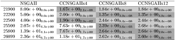
 on all instances.
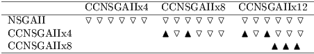
 (Mean and standard deviation).
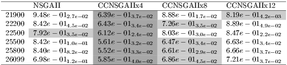
 on all instances.
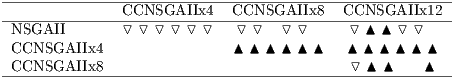
This article has proposed to apply for the first time a parallel asynchronous cooperative coevolutionary NSGAII (CCNSGAII) on a real-world problem, i.e., the injection network problem in VANETs. Three parallel CCNSGAII configurations were studied, just differing on the number of subpopulations. The performance of the algorithms has been compared to the standard NSGAII in terms of execution time and solution quality. Experimental results have demonstrated that super-linear speedup has been obtained on all problem instances, with all parallel configurations. In addition, the convergence of the obtained Pareto fronts could be improved with statistical confidence for all cases as well as their diversity for some of them.
Future works will focus on new mechanisms to improve diversity of solutions when a high number of subpopulations is used. Additionally, we will consider using other state-of-the-art MOEAs like SPEA2 and MOCell on the same topology control problem in VANETs.
B. Dorronsoro acknowledges the support offered by the National Research Fund, Luxembourg, AFR contract no 4017742.
[1] C. A. C. Coello, G. B. Lamont, and D. A. Veldhuizen, Evolutionary Algorithms for Solving Multi-Objective Problems. Springer, 2007, second edition.
[2] M. Potter and K. De Jong, “A cooperative coevolutionary approach to function optimization,” in Parallel Problem Solving from Nature (PPSN III). Springer, 1994, pp. 249–257.
[3] A. W. Iorio and X. Li, “A cooperative coevolutionary multiobjective algorithm using non-dominated sorting,” in GECCO (1), 2004, pp. 537–548.
[4] K. C. Tan, Y. J. Yang, and C. K. Goh, “A distributed cooperative coevolutionary algorithm for multiobjective optimization,” IEEE Transactions on Evolutionary Computation, vol. 10, no. 5, pp. 527–549, 2006.
[5] S. Nielsen, B. Dorronsoro, G. Danoy, and P. Bouvry, “Novel efficient asynchronous cooperative co-evolutionary multi-objective algorithms,” in Evolutionary Computation (CEC), 2012 IEEE Congress on, 2012, pp. 1–7.
[6] Y. Pigné, G. Danoy, and P. Bouvry, “A vehicular mobility model based on real traffic counting data,” in Proc. 3rd International Workshop on Communication Technologies for Vehicles (Nets4Cars 2011), vol. 6596. Springer, LNCS, 2011, pp. 131–142.
[7] G. Danoy, J. Schleich, B. Dorronsoro, and P. Bouvry, “Optimising small-world properties in VANETs with a parallel multi-objective coevolutionary algorithm,” in VI Latin American Symposium on High Performance Computing (HPCLatam), 2013, pp. 13–24.
[8] B. Dorronsoro, G. Danoy, A. J. Nebro, and P. Bouvry, “Achieving super-linear performance in parallel multi-objective evolutionary algorithms by means of cooperative coevolution,” Computers & Operations Research, vol. 40, no. 6, pp. 1552 – 1563, 2013. [Online]. Available: http://www.sciencedirect.com/science/article/pii/S030505481100339X
[9] J. Mao, K. Hirasawa, J. Hu, , and J. Murata, “Genetic symbiosis algorithm for multiobjective optimization problem,” in Proceedings of the 2001 Genetic and Evolutionary Computation Conference, San Francisco, California, 2001, pp. 267–274.
[10] N. Keerativuttitumrong, N. Chaiyaratana, and V. Varavithya, “Multi-objective co-operative co-evolutionary genetic algorithm,” in International Conference on Parallel Problem Solving From Nature PPSN, ser. Lecture Notes in Computer Science (LNCS), vol. 2439. Springer-Verlag, 2002, pp. 288–297.
[11] E. Zitzler, K. Deb, and L. Thiele, “Comparison of multiobjective evolutionary algorithms: Empirical results,” Evolutionary Computation, vol. 8, no. 2, pp. 173–195, 2000.
[12] K. Maneeratana, K. Boonlong, and N. Chaiyaratana, “Multi-objective optimisation by co-operative co-evolution,” in PPSN, 2004, pp. 772–781.
[13] E. Zitzler, M. Laumanns, and L. Thiele, “SPEA2: Improving the strength Pareto evolutionary algorithm,” Computer Engineering and Networks Laboratory (TIK), ETH Zurich, Tech. Rep. 103, 2001.
[14] A. Nebro, J. Durillo, F. Luna, B. Dorronsoro, and E. Alba, “MOCell: A cellular genetic algorithm for multiobjective optimization,” International Journal of Intelligent Systems, vol. 24, pp. 726–746, 2009.
[15] K. Deb, L. Thiele, M. Laumanns, and E. Zitzler, “Scalable multi-objective optimization test problems,” in Congress on Evolutionary Computation (CEC), 2002, pp. 825–830.
[16] K. Deb, A. Pratap, S. Agarwal, and T. Meyarivan, “A fast and elitist multiobjective genetic algorithm: Nsga-ii,” Evolutionary Computation, IEEE Transactions on, vol. 6, no. 2, pp. 182–197, 2002.
[17] J. Schleich, G. Danoy, B. Dorronsoro, and P. Bouvry, “An overlay approach for optimising small-world properties in vanets,” in Applications of Evolutionary Computation, ser. Lecture Notes in Computer Science, A. Esparcia-Alcázar, Ed. Springer Berlin Heidelberg, 2013, vol. 7835, pp. 32–41. [Online]. Available: http://dx.doi.org/10.1007/978-3-642-37192-9_4
[18] D. J. Watts and S. H. Strogatz, “Collective dynamics of small-world networks,” Nature, vol. 393, no. 6684, pp. 440–442, 1998.

