Energy Consumption of Clocks Synchronization on a Routing Algorithm for Sensor Networks

 

 

Enrique Giandomenico, Estela D’Agostino, Javier Belmonte, Rosa Corti, Roberto  Martínez

Universidad Nacional de Rosario, Facultad de Ciencias Exactas, Ingeniería y Agrimensura

Rosario, Argentina, 2000

{giandome, estelad, belmonte, rcorti, romamar}@fceia.unr.edu.ar

 

Abstract

Cluditem is a routing algorithm for wireless sensor networks developed for applications of environmental monitoring with periodic measurement of variables. These applications tolerate a maximum phase shift of the clocks of nodes in the order of milliseconds. This paper proposes two centralized synchronization schemes that introduce a limited processing load.  The objective of the work was to assess the impact on the energy consumption of the incorporation of synchronization techniques described. Simulations of the full communication protocol were conducted in the NS2 environment and a comparative study of results was performed. This study showed that the first proposed schema is more convenient with respect to energy consumption, when the area to monitor has reduced dimensions. On the other hand, the second scheme, although it permits to work in larger areas, introduces a decrease in the network lifetime in the order of 14%.  

Spanish abstract

Cluditem es un algoritmo de encaminamiento para redes de sensores desarrollado para aplicaciones de supervisión ambiental con medición periódica de variables. Estas aplicaciones admiten un desfasaje máximo de los relojes de los nodos del orden de los milisegundos. En este paper se proponen dos esquemas de sincronización centralizados que introducen una carga de procesamiento acotado.  El objetivo del trabajo realizado fue evaluar el impacto sobre el consumo de energía de la incorporación de las técnicas de sincronización descriptas. Se efectuaron ensayos de simulación del protocolo de comunicaciones completo en el ambiente NS2 y se realizó un estudio comparativo de los resultados obtenidos. Este análisis mostró que el primer esquema propuesto resulta más conveniente, respecto del consumo de energía, cuando el área a supervisar posee dimensiones reducidas. Por el contrario, el segundo esquema, aunque permite trabajar en áreas más extensas, introduce, respecto del primero, una disminución de la vida útil de la red del orden del 14%. 

 

                Keywords:  Wireless sensor networks, Synchronization algorithms, Energy consumption, Clustering algorithms.

           

Spanish keywords:  Redes inalámbricas de sensores, Algoritmos de sincronización, Consumo de energía, Algoritmos basados en clusters

 

Received 2012-05-30, Revised 2013-01-15, Accepted 2013-01-15

 

 

 

 

1 Introduction

Wireless smart sensors networks (WSSN) are used to measure variables in the environment with the purpose of carrying out monitoring and control environments and varied activities. They consist of nodes that self-organize to adapt themselves to changing topologies and collaborate with each other to send their measurements to one or more base stations also known as sink nodes. Communication between devices is wireless and RF transmission is the most widely used (1). Fig. 1 shows the scheme of a network of sensors whose single base station, responsible for final processing of the information, is located outside the area under study.

The WSSN are integrated in applications of different kind: industrial, medical, preservation of the natural environment, disaster assistance, creation of intelligent facilities, and others. In many of these applications, the acquisition of the variables of interest must take place in hostile and/or distant locations that make it very difficult the wiring and maintenance of measurement devices (2). Therefore, to ensure a lifetime according to the needs, the nodes must have a significant degree of autonomy and then to save as much energy as they can. The availability of resources in each device for storage, processing capacity and communication is limited not only by the available energy, but also by requirements like small size and low costs for the nodes, found in many applications. These distinctive features of the WSSN have great impact on the design of the software and hardware components of sensor devices (1) (3).

Techniques for time synchronization, some of them long-tested with very good performance, have a long history of research in the area of distributed systems but they cannot be used in wireless sensor networks for the reasons previously mentioned (1). The addition of dedicated hardware in the nodes to synchronize with external sources, such as the addition of GPS receiver, is prohibitive considering the existing restrictions for devices, and often expensive. Moreover, synchronization algorithms whose complexity may collide with the limitations of the hardware platform that will support them cannot be included. For these reasons, in the same way that has occurred in the areas of algorithms of routing, processing of information and hardware platforms, wireless smart sensors networks have required specific developments to address the problem of the time synchronization (4) (5) (6).

Figure 1: WSSN scheme

The WSSN usually track phenomena and events of the environment for which time plays a very important role in dealing with following tasks (7):

• Data collection: measurements must be done in certain periods, and it is often necessary to know the time in which they were acquired to be able to reconstruct the history of the phenomenon under study. For example, for supervision of civil works and follow-up of patients health parameters.
• Coordination of tasks: the nodes must perform actions following a certain pattern and, if possible, in a coordinated manner. An example is when transceivers are switched off to save power, and then the nodes must come into activity within a certain period of time. If the nodes clocks are considerably out of phase, many of the exchanged messages will be lost.
• Time-dependent calculations: among the variables to measure is the time that is required to perform different calculations. The accuracy of these depends on the accuracy of the measured value.

The clocks of devices are independent of each other and their values may be different. This situation often cause difficulties in the aforementioned tasks (8). The difference between the values of the clocks in the nodes is due to:

• Devices start their activity at different instants of time.
• The crystals of the clocks are not the same for reasons of manufacturing (skew), which causes the values to become out of phase in time.
• Working frequency is sensitive to environmental variations, like temperature, introducing an error by frequency variations (9).

The variation in the frequency of an oscillator, caused by the two last mentioned effects, produce the so-called clock drift and introduce differences in local times that may be very significant. In addition to the different clock values due to problems inherent in the characteristics of the watches, phase shift can occur during transmissions. Processes for time determination are affected by delays in the propagation of messages. The calculation of the time should be done guaranteeing specific margins of accuracy, but due to the nature not deterministic of the processes involved, reliable levels of precision cannot be reached. In this sense, it should be noted that the latency in the transmission channel is due to the following causes (8):

• Dispatch time: is the time consumed by the transmitter in assembling the message to send
• Access time: is the time that elapses until access to the channel
• Propagation time: is the time that the message takes to travel from the transmitter to the receiver
• Reception time: includes the time between when the receiver receives the message and processes it (4).

Some applications of sensor networks are strict with respect to the notion of time and need to synchronize the devices with an accuracy of a few tens of microseconds. In environmental monitoring applications with periodic measurement of variables to which this work focuses, the notion of absolute time in the nodes is not necessary and a difference of milliseconds between the clocks can be accepted. The reason for the relaxation of the synchronization requirements in this type of application is based on the behavior that is expected of the network. All nodes collect the information of interest after a period T, whose duration depends on each application in particular, and send it to the base station performing what is known as batches of measurement or data acquisition. To achieve a good performance in this job, it is enough to guarantee a maximum phase shift in each batch of measurements in order to take security factors, and in this way sequencing phases of operation in each of the batches of data acquisition. The definition of tasks and its temporal distribution is the responsibility of the routing algorithms, which sets the paths to be used to send information to the base station applying topology control techniques suitable for sensor networks design requirements (5).

This work presents different approaches in the time synchronization for the algorithm of routing Cluditem, which is oriented to applications of environmental monitoring with periodic measurement of variables. The objective is to assess the impact that the incorporation of proposed synchronization techniques has on energy consumption, in a sensor network based on Cluditem.

The rest of the work is organized in the following way: Section 2 describes how Cluditem algorithm works. Section 3 classifies synchronization techniques for WSSN, highlighting the most commonly used. Section 4 includes a report of other works related with the presented here and in Section 5 the synchronization techniques proposed for Cluditem are analyzed and simulation results presented. Finally, in Section 6 conclusions are revealed and future work lines are set out.

 

2 Description of Cluditem

Cluditem is a hierarchical routing algorithm for sensor networks oriented towards applications of environmental monitoring with periodic data acquisition. In these applications the accent is placed on the quality of information and not on the speed of response, so the control of latency is not a priority. In particular, in the development of the algorithm, applications quality of service (QoS) was defined as a maximum permissible percentage of loss of information. This requirement is typical in applications that need information about the whole region where the network has been deployed to obtain a map of variation of the variables in order to build a model of the behavior of the system, make decisions or carry out corrective actions. Therefore, the network lifetime is defined as the number of batches of measurement can be performed respecting the defined QoS.

The structure of the routing that Cluditem defines uses clusters, therefore exist two types of nodes in the network, the header (CH) that coordinates a group of nodes and the member nodes or common nodes (CN) (10). The nodes of the network are fixed and homogenous in their hardware platform and available resources, differing in its functionality. In this sense, the network works with two transmission radius, a reduced one for the CN transmissions, and another of greater range for communication of the headers. The specific transmission power settings are set for each particular application.

The algorithm divides its operation in three distinct stages that are repeated periodically during the entire life of the network. The first one establish the routing tree, during the second data are sent to the sink, and in the third all the nodes of the network remain in low power state. This last stage is related to an important feature of Cluditem which specifies to shutdown devices all the time possible, while maintaining the QoS established in response to the requirement of autonomy of operation. It is important to note that since Cluditem is a hierarchical distributed algorithm, the transceivers shutdown is defined by each node using its own clock. It is therefore required to synchronize the clocks of the members of the network for the message exchange to be effective. The development of the algorithm was performed assuming a maximum inter and intra cluster clocks phase shift,  so it must be guaranteed with the synchronization  technique  to add.

Communication between the nodes of a network based on Cluditem is multi hop and for the lower layers of the communication protocol the IEEE 802.15.4 standard was adopted which is recommended for this type of networks. In this sense, the algorithm combines CSMA/CA (Carrier Sense Multiple Access/Collision Avoidance) without slots in the MAC layer with a TDMA (Time Division Multiple Access) scheme defined at the level of routing in order to reduce intra and inter cluster collisions. The following sections summarize the most important aspects of the operation of the algorithm, on which a complete and detailed description can be found in (11).

 

2.1 Definition of Routing Tree

The routing that defines Cluditem is based on a structure with two hierarchical levels. The first consists of a set of clusters, with a single coordinator to which the near nodes report to, and the second consists of a tree formed by the header nodes, which summarizes the information collected by their children and cooperate with each other to make it reach the base station (12).

The CHs are nodes with large number of responsibilities, which remain active more time and transmit with greater range. Therefore, they consume more energy than the CNs in each batch of measurement. However, the nodes of a Cluditem network are homogeneous in terms of their resources, so a technique of periodic rotation of roles among nodes has been incorporated to balance energy consumption among the network members.

In this sense, the reconfiguration of the routing tree, which includes reassign the role of CH, occurs periodically every X batches of measurement. Fig. 2 shows the operating stages of Cluditem that repeat during the entire lifetime of the network. In it, TRD is the routing definition phase, TDATA corresponds to sending measurements to the sink and TSLEEP represents the period in which the nodes remain in low power state. Also highlights that the reconfiguration of the routing structure (TRD), is performed every X batches of data collection.

Figure 2: Cluditem operating stages

2.1.1 Definition of the Structure of Clusters

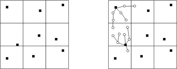
The definition of clusters starts with the postulation of the nodes that will assume the role of CH in the current reconfiguration. This is an important aspect in the design of the algorithm, since a good distribution and an appropriate amount of headers is a milestone of the algorithm in order to the network may perform its functions properly. To achieve this, Cluditem divides the area to monitor on the basis of a virtual grid and uses it during the process of choosing CHs and clusters definitions. Fig. 3 shows a sample definition of clusters in a network where the area to monitor is divided into a virtual grid of 9 cells.

Figure 3: Use of virtual grid to define clusters (a) Generic grid with CH (b) Example of clusters set up

Once its nomination is done, the headers transmit a message called cluster structure message (CS) with the format shown in Fig. 4. Each node that listens to a CH, and decides to join the cluster that coordinates this CH, forwards the message replacing the transmitter and transmitter level fields with its own data, so the neighbors can adopt it as a link node (LN) in the cluster. The level of the node in a cluster represents the amount of hops separating it from its header. Therefore, when choosing a LN each node defines its level by adding 1 to the level of its LN. As you might expect, the CH are level 0.

Figure 4: Cluster structure message (CS)

2.1.2 Headers Tree Definition

The second level of the routing tree defines the communication path to the sink of all headers, with the aim that clusters information reaches the base station. Communication between the CHs and the sink can be multi hop, because the area to monitor is resizable and the transmission radius of the CH is limited.

The definition of the headers tree begins with a message that the base station sends to the network, with a radius of transmission equal to that used by the CH to communicate with each other. The nodes that hear this message directly record this situation. Among these ones, those who assumed the role of header during the cluster definition phase sent a message of assembly of CHs tree (CHT), announcing that the base station is within its transmission radius and that therefore its level is 1. The structure of the CHT message is shown in Fig. 5. From its data each CH choose their link node as the header that it hear with the lowest transmitter level. It then forwards the CHT message communicating its identity and its level to allow other nodes to choose it as LN in the tree.

Figure 5: CHs tree message

2.2 Sending Data to Base Station

The stage for sending data takes place during T_DATA and is carried out in two phases: in the first, length T_SD, the common nodes send their measurements to its cluster header, and in the second, that runs during T_SA, the CH use headers tree to make an aggregated message reach the base station. This message summarizes the information gathered by the CH from the cluster it coordinates. Data sending occurs after the definition of the routing tree (T_RD) if it is reconfiguration batch, or at the beginning of the period T of gathering information in a batch of exclusive transmission of measurements (13).

Fig. 6 shows the phases of information transmission and highlights that the intra and inter cluster data transmission is done fulfilling a TDMA scheme in each one of them, to prevent collisions. In the same, TSLOT_SD and TSLOT_SA  represent time slots adopted for sending data and aggregated data, respectively.

Figure 6: Detail of data transmission stages

During TSD, the ordinary nodes send measurements to their header using a data message, whose structure is shown in Fig. 7.

Figure 7: Format of a data message

At the end of TSD, headers join an aggregated message with its cluster information and send it using the CHs tree up to the base station. Fig. 8 shows the structure of the message that headers transmit towards the sink node. When the data collection batch is done, the network repeats the described operation until it exhausts its useful life because it is unable to satisfy the established requirements of QoS

Figure 8: Format of aggregated message

2.3 Consumption of the Algorithm without Clock Synchronization

During the entire lifetime of the network, Cluditem performs, on a regular basis, batches of measurements of the environment variables of duration T. The set of batches carried out using the same routing structure has been termed round. As already mentioned, a batch may include the redefinition of the routing prior to proceed with sending information (RDB), or may be for data transmission only (DB). It was defined that each round includes a batch of reconfiguration followed by several batches without reconfiguration. The number of batches included in one round is called X, as mentioned in Subsection 2.1.

The reconfiguration of the network implies a higher consumption of energy so it is desirable to reduce the number of times it occurs. On the other hand, to avoid premature disconnections by keeping consumption balanced among members of the network, it is necessary to rotate the role of header, redefining the routing. Based on these considerations, the ideal situation corresponds to all nodes assuming the role of CH only once during the system lifetime, consuming all their reserves of energy (EIN ).To reach a compromise solution as close as possible to the ideal case and distribute the CH in the area under study, Cluditem uses a virtual grid. It consists of cells with the same number n of nodes each that, in the phase of definition of clusters, support to the election of candidates to header as described in Subsection 2.1.1. In this sense, during the lifetime of the network, Cluditem performs n redefinitions of the routing by implementing strategies to make the average number of times a node assumes the role of CH (Z) close to the ideal value (Z = 1).  The energy consumed by a node during a round depends on the role that it assumes since CHs require more resources than CNs. Therefore, the consumption in a round of a CH (ECHRC) responds to the expression (1), while consumption in a round of a CN (ECNRC) to the expression (2).

 

 

 

ECHRC = ECHBR + (X - 1) . ECHBWR	(1)
ECNRC = ECNBR + (X - 1) . ECNBWR	(2)

 

Where:

·          E_CHBR: Energy consumed by a Cluster Header node in a Batch with Reconfiguration.

·          E_CHBWR: Energy consumed by a Cluster Header node in a Batch Without Reconfiguration

·          E_CNBR: Energy consumed by a Common Node in a Batch with Reconfiguration

·          E_CNBWR: Energy consumed by a common node in a batch without reconfiguration

 

The node consumption in the n rounds that it performs in its lifetime must be equal to the energy the elements that feeds it can provide (EIN), as noted in expression (3).

 

EIN = Z . ECHRC + (n - Z) . ECNRC

(3)

Once set the value of EIN, the most appropriate value of X can be obtained as a function of n, Z and the energy consumed by each node type in each batch type. To perform the analysis of results of Section 5, the values relating to the consumption of nodes and the average value Z were achieved by successive approximations, based on the simulation of the algorithm in NS2.

 

3 Synchronization Schemes for WSSN

The synchronization algorithms commonly used in sensor networks are classified, according to working modes, as proactive or reactive. Proactive algorithms repeat periodically the synchronization tasks during the entire lifetime of the system with the aim of maintaining the phase shift of the clocks bounded. For example, a reference node periodically sends the value of its local time in a message and others nodes in its operating range estimate their phase shift based on its local time and the received value. On the other hand, reactive algorithms proceed with synchronization only when certain events occur (7). In addition, synchronization schemes are divided, under other criteria, in adaptive and non-adaptive. The first ones can modify important parameters in the synchronization procedure, such as periodicity, in response to changes in the network or in the environment; the last ones does not modify the algorithm at any time. The techniques of synchronization proposed in this work belong to the group of proactive - no adaptive algorithms.

Synchronization schemes introduce computational overhead, increase traffic on the network because of added message exchanges and rise energy consumption. Therefore, a balance must be maintained between the costs of incorporating synchronization in WSSN and the need to maintain the time errors due to clock phase shifts bounded.

Among the most commonly used synchronization procedures we can mention (7):

·           Transmitter-receiver synchronization. A node sends the value of its clock in a message. When another node receives it, reads its own clock and calculates the phase shift with respect to the transmitter. The propagation time is generally disregarded.

·           Peer-to-peer synchronization. It consists in an exchange of messages between two nodes, placing in each message sent the value of its own clock. They take into account the propagation time that they assume equal in both directions, and consider that the difference between their clocks is kept constant during all the course of transmission. In this way, doing a simple calculation, the device gets the phase shift in respect of its neighbor.

·           Reference transmission. The assumptions considered by the above method does not always are true and to decrease the error a reference node is established and all nodes that must be synchronized listen to it.

 

4 Related Work

Reference Broadcast Synchronization (RBS) (14) and Timing-sync Protocol for Sensor Networks (TPSN) (15) are the most used synchronization algorithms. Cluditem uses clusters in the definition of the routing structure of the network, so we can relate it to the algorithm Scalable Lightweight Time Synchronization Protocol for WSN (SLTP) which includes the definition of clusters during the procedure of synchronization (16). 

In the RBS algorithm a reference node sends a message to its neighbors through a special synchronization channel, without attaching any time value in the message. The neighbors use the reception time to synchronize, i.e. it is   receiver-receiver synchronization algorithm. The problems that RBS can arise have to do with the number of neighbors who hear, i.e. how many nodes are going to synchronize based on the receipt of this message. As the number of nodes increases, it is possible that one does not reach the synchronization. For this reason, the synchronization message is sent periodically (14).

TPSN protocol works in two stages; in the first, called discovery, a hierarchical structure is defined and in the second, named synchronization, a transmitter-receiver scheme is used. The hierarchical structure has a single node of level 0 and any node of i level can communicate with at least one node of i-1level (15).

SLTP algorithm has two phases of work, of configuration and synchronization. In the configuration stage, the headers of all clusters are statically or dynamically set. In a static configuration, a flag is used to define the CH. This flag, which is transmitted in the message exchanged between nodes, indicates whether the sending node is a cluster header or a common node. Each node that receives a message from a common node becomes CH and forwards the package indicating its new condition. Common nodes members of a cluster recognize their header node and, if they have more than one, they turn into gateway nodes. Once static configuration is completed, device synchronization starts. On the other hand, if a dynamic configuration is performed, the structure of clusters changes over time and only the CHs are defined in the first stage. Common nodes and gateways are set in the synchronization stage. In this last stage, the CHs are responsible for sending the synchronization message containing their local clocks times. Cluster member nodes calculate their oscillation frequency and phase shift based on the value received from their CHs (16).

These synchronization protocols and several others look for higher accuracies, that is to say, to keep the clocks of the nodes of the networks as synchronized as possible to give to the nodes measurements a precise time correlation. Cluditem does not need a high level of synchronization since it is used mainly for environment measurements and it only requires synchronization because of its routing schema and energy saving mechanisms. In the following paragraphs these aspects will be fully explicit.

 

5 Synchronization in Cluditem

Cluditem was developed for applications that admit a phase shift on the order of milliseconds. Therefore, to achieve a good performance of the algorithm, lightweight synchronization techniques that introduce a bounded processing load have been proposed and tested, allowing then to reach the established requirements.

The collecting batches have a duration T of the order of 10 or 15 minutes.  The nodes of the network remain in activity over a period of a few seconds at the beginning of each batch, and then enter into low power state until met T. In this sense, it was determined that it was sufficient to perform the synchronization of local clocks only once at the beginning of each batch, which was verified through the results of the simulations. The proposed technics are centralized, since the synchronization scheme is initiated by the sink node, having considered various options based on the inherent variations of the scenarios of the applications and on the obtained simulation results.

The operation of Cluditem was analyzed by using the NS2 v2.30 in all the tests described in this paper. This discrete event simulator is aimed to the analysis of protocols for communication networks and was developed in the framework of the project VINT (Virtual InterNetwork Testbed) (17).  It is a working tool widely known and used in both wired and wireless networks (18).

 

5.1 Working Environment and Simulation Scenario

In the NS2 environment it is possible to define the complete communication protocol stack, allowing simulating the behavior of the routing algorithms in conditions close to reality. For the lower layers of CLUDITEM it was chosen the IEEE 802.15.4 standard, which specifies the physical and media access layers of the protocol stack. In this sense, Fig. 9 outlines the implementation.

Figure 9: Protocol communication implemented in NS2

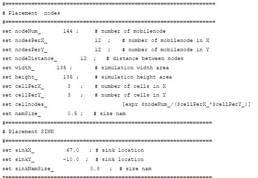
The simulation scenario for all tests was defined as a square area with a side of 135 meters divided into 9 cells, with 16 nodes each, these ones separated 12 meters of each other, and a single base station with unlimited energy located outside the area under study. These chosen values are compatible with applications of interest, but also the characteristics of the scenario were associated with parameters to allow the adjustment of the operation of the algorithm for particular cases, as shown in the script of Fig. 10.

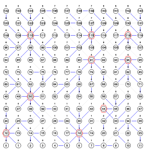
Fig. 11 shows the chosen simulation scenario as presented by the Nam graphical tool associated with the simulator. This figure shows the 144 nodes of the network, divided into 9 cells of the virtual grid. Fig. 11 also illustrates the definition of clusters in the network, made by the algorithm in a batch with reconfiguration. In it, the CHs are highlighted and the generated structure can be seen looking at the lines indicating the LN of each device in its cluster. The base station is outside the plotted area.

Figure 10: Definition of simulation scenario in NS2

Figure 11: Example of definition of structure of clusters

5.2 Results Considering Perfect Clocks

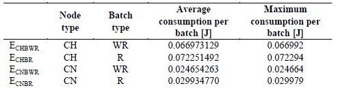
In these trials, it was not taken into account the clocks drift, therefore the initial maximum deviation of 60 milliseconds among devices local times remains constant throughout the entire lifetime of the network. According to these conditions, simulations of operation consisted of 16 rounds (n = 16) of 16 batch of measurements each (X = 16). The value of n corresponds to the number of devices in each square of the grid, and its value was established as part of the simulation scenario described in the previous section. The value of X was defined based on the results of simulations starting with an initial X value and successive adjustments. The trials results allowed to determine the energy consumed by nodes depending on the assumed role and the type of batch made (E_CHBR, E_CHBWR, E_CNBR y E_CNBWR), as well as the value of Z, average times that a node assumes the role of CH during the lifetime of the network.  From these values, expressions (1), (2) and (3) were used to get X. It should be noted that the initial energy of the nodes E_IN was established in a very low value, to limit the simulation time. Table 1 shows the results for the average and maximum consumption of nodes of the network.

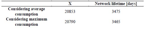
The next step was to determine, in days, the lifetime of the network, considering that each device counts with energy of an AA battery. Consumption values of Table 1 were used for this, and the value of 15 minutes was adopted as the duration of each batch of measurements (T = 15 min).  The results of the calculations are presented in Table 2.

Table 1: Values ​​of energy consumed for drift-free clocks obtained by simulation (X=16)

Table 2: Batches per round and network lifetime for drift-free clocks (E_IN corresponds to an AA battery)

5.3 Results Considering Clock Drift

These tests were performed considering a clock drift value for the nodes of the network varying between -40 and +40 parts per million, in the worst case. Once established, the clock drift remains constant during the entire simulation. Clock drift causes that the phase shift among the times of the nodes varies permanently. Therefore, for the group of applications of interest, it is necessary to periodically synchronize the clocks of devices.

The two proposed schemes of synchronization are initiated by the base station. At the end of period T, all nodes assume the active status to start a batch of measurements. Local clocks are out of phased and therefore, the nodes instead of automatically initiate their activities, remain waiting for a signal of synchronism from the sink. Thus, at the beginning of each batch, all clocks get synchronized so that the sequence of planned tasks runs effectively. The time that elapses from the moment the nodes are activated at the beginning of each batch and the moment in which they receive the signal of synchronism of the sink, increases the total time that the nodes are active and therefore the energy consumed. In order to minimize this effect, the sink must send the sync message as soon as possible from the moment it was sure that all nodes are active and able to receive it.

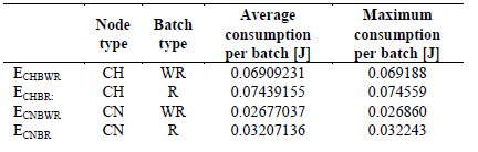
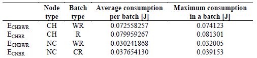
Table 3: Values of energy consumed in the 1^st synchronization scheme, obtained by simulation

The first proposed scheme assumes that the sync message issued by the base station reaches to all nodes on the network, i.e. that the transmission radius of the sink is such that all devices can directly receive their transmissions. With this scheme, the sync message reaches all nodes almost simultaneously since the only phase shift present is the one due to the different distances to travel to reach each of the devices, and this is considered negligible. However, the incorporation of this scheme into the operation of Cluditem rises the time the nodes should remain active because it adds, at the beginning of each batch, a period for clocks synchronization. Therefore, for the tests done, the value of X was recalculated following the procedure described in the preceding paragraph and maintaining the initial energy of the nodes EIN used for clocks without drift. The obtained value was founded to be the same (X = 16), which indicates that the introduced increase of the period of activity, allows to approach the ideal situation in which all nodes in the network assumes the role of CH in a rotation, without diminishing the number of batches in a round. To quantitatively evaluate the influence of increased activity in the nodes, the values of energy consumed when considering ideal drift-free clocks and those founded including the proposed synchronization scheme can be compared. These are presented in Tables 1 and 3 respectively. In this sense, Fig. 12 shows that the impact on the consumption of the CHs is on the order of 3%, while for the CNs fluctuates between 7% and 8.5%. The greater impact on the consumption of the CNs is explained because the synchronization scheme defines the addition of a fixed period at the beginning of each batch. Therefore, this one influences percentage-wise much more on consumption of the common nodes which remain active, in all the batches, a period significantly less than the CHs.

Figure 12: Increase of consumption introduced by the 1^st synchronization scheme with respect to drift-free clocks

Table 4 presents the values of X and the network lifetime when incorporating this synchronism scheme, taking EIN as the value corresponding to an AA battery and the consumption of Table 3. Comparing the 3465 days of useful life of the system, considering maximum consumption, with the value obtained in Table 2 when working with clocks without drift, we can appreciate the network lifetime decreases by 7.3%.

Table 4: Batches per round and network lifetime for the 1 ^st synchronization scheme (E_IN for an AA battery)

The area to monitor depends on the application and its dimensions can vary considerably. Therefore, it may not be feasible that base station messages reach all nodes directly. For this reason, the second synchronization scheme is proposed. In it, the sink transmits the sync message with the same transmission power used by CHs. Each node, regardless of whether is header or not, when it receives the message from the base station, forwards it only once and starts the tasks corresponding to the current batch type. If it receives a new sync message due to broadcasts of its neighbors, it discards it. It is important to note that this synchronization scheme has two drawbacks.

a)         The sync message arrives to the nodes at different times. Since a node receives the message until it retransmits it, a period elapses and its duration varies according to the conditions present in the network. In addition, there will be nodes that receive the message after forwarded by multiple devices, so they synchronize out of phase from those who received it before. Fig. 13 shows on the y axis the percentage of nodes whose phase shift is less than or equal to that indicated on the x axis. In this sense, 16% of the nodes synchronize 2.53 milliseconds after the base station issued its synchronization message and all nodes are synchronized before 4.51 milliseconds.

b)        The traffic of sync messages is affected by the possibility of collisions, which causes some of the nodes of the network do not receive the message at all. These ones do not start the activities corresponding to the current batch of measurements and therefore they are not involved in the sending of information to the base station. This situation is particularly serious if nodes that are isolated have, in the current batch, the role of headers since the measurements collected by all CN members of the clusters they lead will be lost.

The second considered work scheme requires a longer period to synchronize the nodes of the network because of the variable times involved, as described in point a). In this sense, the total time that each node must remain in the active state in each batch of measurement increases. This results in higher energy consumption. Furthermore, to reduce the impact of the problem described in point b), it was decided that the base station emits two sync messages in a short time. Nodes forward and get synchronized on first receipt of a sync message from the base station. Therefore, those devices that receive the two transmissions emitted by the sink ignore the second. The scheme considers the addition of a fixed period for synchronization of the nodes at the beginning of each batch of measurement. This implies that all devices are synchronized when they start their activities of the current batch, regardless of whether they received the first or the second message from the base station.

Figure 13: Number of nodes (%) whose phase shift is less than or equal to that indicated on the x axis

Table 5: Values of energy consumed in the 2^nd synchronization scheme, obtained by simulation(X=14)

Figure 14: Increase of consumption introduced by the 2^nd synchronization scheme with respect to drift-free clocks

The tests were performed with the same initial energy in the nodes EIN used in previous cases. However, this second scheme adds a synchronization period longer than the corresponding to the first scheme. Therefore, the recalculation of X from EIN and consumption values of nodes by role and batch type presented in Table 5, resulted in a value of X = 14. This indicates a greater impact on the energy consumption of the nodes of the network, as shown in the Fig. 14. As for the previous scheme, Fig. 14 shows that the relative increase in the consumption of the CHs (8.3% to 10.6%) is lower than the one suffered by the CNs (22.6% to 25.7%). The greater impact on the consumption of the CNs is explained for the same reasons mentioned when analyzing the first scheme.

Finally, it was obtained the value of X and the network lifetime considering that the initial energy of the nodes EIN is provided by an AA battery. Results are shown in Table 6. In this case, it can be seen that the system lifetime is reduced by a 21.08% when using the 2nd synchronization scheme.

Table 6: Batches per round and network lifetime for the 2 ^nd synchronization scheme (E_IN corresponds to an AA battery)

6 Conclusions and Future Work

This work introduced two centralized synchronization schemes for Cluditem, a routing algorithm oriented to applications of environmental monitoring with periodic measurement of variables. Applications of interest admit differences on local clocks on the order of milliseconds. The proposed techniques, whose performance was evaluated by simulation, introduce a reduced processing load, although they require that the nodes perform additional tasks and remain more time active, raising their energy consumption.

The first scheme analyzed is more favorable with reference to the increase of energy consumption in devices, but it requires that the base station transmissions reach all nodes on the network. Therefore, their use is recommended only if the dimensions of the area to monitor are compatible with that requirement. If this is not the case, one must resort to the second scheme that reduces the useful life of the network by 14% more than the first scheme described.

The proposed schemas constitute an advantage when comparing with other synchronization protocols commonly used in WSN because they allow to maximize the network lifetime for Cluditem application scenarios. However, these techniques have the weakness that they can not be implemented in domains where high accuracy is needed.

Currently we are working on the implementation of Cluditem in a hardware platform, incorporating synchronization schemes discussed in this paper. The devices used are nodes for wireless sensors networks of type System on Chip (SoC) from Texas Instruments (CC2530 and CC2531) (19). The objective is to create a network of approximately 25 nodes for in-field testing of scenarios compatible with the selected applications.

References

(1)          J. Yick, B. Mukherjee and D. Ghosal, “Wireless sensor network survey,”  Computer Networks: The International Journal of Computer and Telecommunications Networking, vol. 52, pp. 2292-2330, Aug. 2008.

(2)          C. F. García Hernández, P. H. Ibargüengoytia González,  J. García Hernández and  J.A. Pérez Díaz,  “Wireless Sensor Networks and Applications: a Survey,” International Journal of Computer Science and Network Security IJCSNS, vol. 3,  pp. 264-273, March 2007.

(3)          C. Buratti, A. Conti, D. Dardari and R. Verdone, “An Overview on Wireless Sensor Networks Technology and Evolution,” Sensors, vol. 9, pp. 6869-6896, Aug. 2009.  http://www.mdpi.com

(4)          W. Ikram, I. Stoianov and N.F. Thornhill,  “Towards a Radio-Controlled Time Synchronized Wireless Sensor Network: A Work in-Progress Paper,” in Proc. IEEE Conference on Emerging Technologies and Factory Automation (ETFA), Bilbao, Spain, Sept. 2010, pp. 1-4.

(5)          S.K. Singh, M.P. Singh and D.K. Singh, “Routing protocols in wireless networks – A survey,” International Journal of Computer Science & Engineering Survey (IJCSES), vol. 1, pp. 63-83, Nov. 2010.

(6)          Z. Pei, Z. Deng, B. Yang and X. Cheng, “Application-Oriented Wireless Sensor Network Communication Protocols and Hardware Platforms: a Survey,” in Proc. IEEE International Conference On Industrial Technology, Chengdu, China, Apr. 2008, pp. 1-6.

(7)          A. Ageev, “Time Synchronization and Energy Efficiency in Wireless Sensor Networks,” PhD Dissertation, International Doctorate School in Information and Communication Technologies, Universit_a degli Studi di Trento, Italy, Mar.  2010.

(8)          I. Rhee, J. Lee, J. Kim, E. Serpedin and Y. Wu, “Clock Synchronization in Wireless Sensor Networks: An Overview,” Sensors, vol. 9, pp. 56-85, Jan. 2009. http://www.mdpi.com

(9)          R. Prakash and N. Kendall, “Time Synchronization in Wireless Sensor Networks: a Survey,” International Journal of UbiComp (IJU), vol. 1, No. 2, pp. 92-102, Apr. 2010.

(10)      A. Abbasi  and M. Younis, “A survey on clustering algorithms for wireless sensor networks,” Computer Communications, vol. 30, pp. 2826-2941, Jun. 2007.

(11)      R. Corti, Clustering dinámico para tiempo de encendido mínimo en redes de sensores inalámbricas CLUDITEM, 1a ed.,  La Plata : Universidad Nacional de La Plata, 2012, E-Book. http://sedici.unlp.edu.ar/handle/10915/4209

(12)      R. Corti, E. D’Agostino, E. Giandomenico, J. Belmonte y R. Martinez, “Clustering Dinámico para Tiempo de Encendido Mínimo en Redes Inalámbricas de Sensores (CLUDITEM) Análisis de la  Definición de Clusters,” in Proc. XXXIV Conferencia Latinoamericana de Informática (CLEI 2008), pp.1229-1238, Santa Fé , Argentina, Sep. 2008.

(13)      R. Corti, E. D’Agostino, E. Giandomenico, R. Martínez y J. Belmonte, “Clustering Dinámico para Tiempo de Encendido Mínimo en Redes Inalámbricas de Sensores (CLUDITEM). Análisis de las fases de envío de datos,” in Proc. XXXVI Conferencia Latinoamericana de Informática (CLEI 2010), pp. 1-13, San Lorenzo, Paraguay, Oct. 2010.

(14)      J. Elson, L. Girod and D. Estrin, “Fine-Grained Network Time Synchronization using Reference Broadcasts,”  in Proc. of the 5th Symposium on Operating Systems Design and Implementation, Boston, Massachusetts, USA, pp. 9–11, Dec. 2002.

(15)      S. Ganeriwal, R. Kumar and M. Srivastava, “Timing-sync Protocol for Sensor Networks,” in Proc. of the 1st International Conference on Embedded Networked Sensor Systems SenSys ’03, pp. 5-7, Los Angeles, USA, Nov. 2003.

(16)      N. G. Sepideh, N. E. Arash, R. Laleh, A. Y. Seyed and D. Mehdi, “SLTP: Scalable Lightweight Time Synchronization or Wireless Sensor Network,” in Proc. of the 3rd international conference on Mobile ad-hoc and sensor networks MSN'07, pp. 536-547, Heidelberg, Germany, 2007.

(17)      The VINT Project. The ns Manual. USA, 2010. http://www.isi.edu/nsnam/ns/doc/ns_doc.pdf

(18)      The Network Simulator - ns-2. http://www.isi.edu/nsnam/ns/

(19)      Texas Instruments. “A True System-on-Chip Solution for 2.4-GHz IEEE 802.15.4 and ZigBee Applications” http://www.ti.com/lit/ds/symlink/cc2530.pdf