Automatic Glaucoma Detection Based on Optic Disc Segmentation and Texture Feature Extraction

1 Introduction

The globalization process has contributed significantly to advances in science, particularly in the area of technology. The benefits obtained of the same are reflected in benefits for humans, such as in eye examinations where in the digital image processing has played a relevant role in the detection of pathologies [1].

The analysis of fundus of the eye images is widely used by the medical community to diagnose eye diseases or diseases that have global effects on the cardiovascular system [2]. There are many eye diseases, which can cause blindness as Cataract, Glaucoma, Diabetic Retinopathy, Conjunctivitis, among others. Glaucoma is a disease that affect the optic nerve gradually, thus leading to a progressive loss of visual field irreversibly. This optic damage is usually caused by increased pressure inside the eye (intraocular pressure) [3].

An alarming feature of glaucoma is the fact of having no symptoms making it increasingly serious and could be noticed only in its most advanced stage. Damage caused by glaucoma can be reduced from the early diagnosis, since there are treatments that prevent the progression of this disease. Therefore, early detection is very important because it prevents total loss of vision.

According to the World Health Organization (World Health Organization) [4], there are about 60 million glaucomatous around the world of which every year there are 2.4 million new cases. A population study conducted in southern region of Brazil randomly selected 1636 people over 40 years, and of these, it was found a prevalence of glaucoma in 3.4% of cases. Also according to this search, 90% of glaucomatous were unaware of their diagnosis [5].

One way to detect glaucoma is through periodic examinations, and to conduct these screenings, specialized equipment is necessary, such as Optical Coherence Tomography (OCT) and Heidelberg Retinal Tomography (HRT). Another way of detection cheaper than conventional screenings it is through the analysis of digital images of fundus of the eye. In this method the ophthalmologist will have to identify through the digital images of fundus of the eye the accumulation of fluid around the Optic Disc (OD) and inform if that retinal image has glaucoma or not [6].

The objective of this work is to create an automatic detection method for Glaucoma through retinal image analysis. For this, we follow five steps: acquisition of image database; segmentation of OD region and evaluation of this segmentation, so that this segmented region to help in the feature extraction, which is the next step; finally we perform the classification of images in glaucomatous or not. Each of these steps will be detailed in Section III. ]]>

2 Work Related

In Kavitha et al. (2010) [7] the segmentation of the OD region and its excavation was made. In this work, the authors carried out the location of the Region of Interest (ROI) so that then is used mathematical morphology techniques for smoothing images and eliminating noise and blood vessels. Finally, active contour algorithm was used for extracting the edge. The difference between the segmentation of the optic disc and its excavation was the image input. In the detection of OD they used the red channel of the image, and for the excavation was used the green channel. The method was tested on 300 images, where these, in almost all the CDR (Cup-to-Disc Ration) was calculated correctly.

In the work of Lim et al. (2015) [8] the segmentation of the OD region and its excavation was made in order to calculate the cup-to-disc ratio. Also in this work, convolutional neural network was used for the removal of blood vessels. Probability maps were generated and these were subjected to a refining procedure that considers the prior knowledge of the retinal structures. Still according to the probability maps, it was possible to obtain an estimate of the accuracy level of segmentation. For the evaluation of the proposed system were used the MESSIDOR and SEED-DB public image databases.

Rajaput et al. (2011) [9] introduced a method for fovea center localization in color eye fundus digital images. This method is based on previous knowledge of OD center and its diameter. In order to OD detection, they applied a histogram equalization to the red channel for contrast enhancement. Then, the authors identified the areas with minimal intensities using the Extended Minima Transform (EMT). The EMT is the regional minima of h-minima transform. They empirically set the h-value (threshold height) to 20. The output was a binary image with the white pixels representing the regional minima in the original image. Regional minima are connected pixels with the same intensity value, whose all external boundary pixels have a higher value. In order to eliminate false detected regions, the authors applied a morphological opening with structuring element disk of radius 8. Finally, the algorithm computed the mean intensities of the identified areas and selected the region with the lowest mean intensity as the OD region. The method was evaluated on 33 retinal images from public DRIVE data set. The experimental results demonstrate that this method is able to detect the fovea center, providing encouraging results.

A similar strategy to our paper was the retinal image detection with Diabetic Retinopathy by Araújo et al. (2013) [10]. In this work, the first step carried out was the segmentation of regions of interest that were exudates. After identifying these regions were extracted color and shape characteristics. The classifier that showed the best result in Diabetic Retinopathy detection was the Multilayer Perceptron (MLP). In this work, it were found results of 88.89% accuracy in exudates identification.

In Danny (2011) [11] the author developed an automatic detection method of Glaucoma from digital images of fundus of the eye. For this, pre-processing techniques and extraction of texture features based on GLCM matrix (Gray-Level Co-Occurrence Matrix) were used. The results indicated that the resources used were clinically significant in the diagnosis of Glaucoma where the proposed system identified the presence of Glaucoma with a precision of 81%.

A method to classify the retinal nerve fiber layer as prone to glaucomatous or not glaucomatous was proposed by Lamani et al. (2014) [12]. To solve the problem of the nerve fiber layer, the authors use descriptor texture and fractal dimension, followed by classification. The color in the fundus of eye images is used for a better analysis of the fiber layer region. The Red channel of the RGB model was used in the image for later extraction of texture features and fractal dimension. The classifier Support Vector Machine (SVM) was used, where it was found that after using this method, in which 40% loss of retinal nerve fibers layer, may be made automatic detection of Glaucoma.

3 Methodology

The method proposed in this paper aims to segment the OD region in retinal images. This segmented region, or region of interest will be used for extraction of texture features in different color models, that then the images be classified as glaucomatous or not.

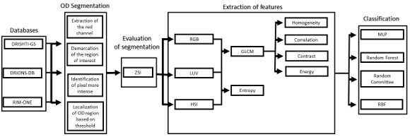
Automatic detection method of Glaucoma in this paper was divided into four phases, as shown in the flowchart in Figure  1. From the acquisition of retinal images, the segmentation of the OD region was made. From the segmented region it was possible to extract texture features using the Grey-Level Cooccurrence Matrix (GLCM) and entropy of images in different color models. Finally, the extracted features are used to classify the image as normal (without Glaucoma) or patient (with Glaucoma).

3.1 Segmentation

The images of the databases were in RGB (Red, Green, Blue) model. As seen in the work of Kavitha et al. (2010) [7], the OD is more easily found on the Red channel of this model, so the images were converted for this channel.

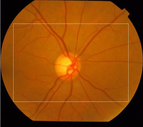
The ROI was obtained to reduce the area where the processing will be made and consequently to reduce the processing time. The region defined refers to the rectangle located in the center of the image, side equal to 3/4 of the original image size. Figure 2 shows an example of ROI defined by the white rectangle.

From the ROI, the central pixel of a 5x5 window was defined as coordinate of the center of OD, that the average intensity of its pixels were the largest of the image. After setting this pixel, it was calculated the radius of the circle of OD. It is worth mentioning that during the calculation of this radius, the pixel previously defined as the center of OD will be modified.

To calculate the estimated radius of OD, it was used a technique based on a threshold. This threshold was found automatically from the found pixel as the center of OD. For this, four radius were drawn: up to the angle of 90^o, down to the angle of 270^o, angle of 0^o to the right and angle of 180^o to the left.

Due to the different intensities of the pixels in the images, a new threshold was calculated for each direction, as being the average between the largest pixel and the lesser color intensity in that direction. Thus, the radius in each direction will be defined as the distance between the pixel of the center of OD and the first pixel that is less than the threshold value.

After radius calculation in each of four directions is made an update of the center of OD that is calculated according to Equations 1 and 2:

(1)

(2)

The final radius of OD is obtained as the arithmetic average of the four radius obtained in the previous step, as shown in Equation 3:

(3)

]]> After the defining of the center and the radius of OD, the circle equation was used to plot the edges of OD, as shown in Equation 4:

(4)

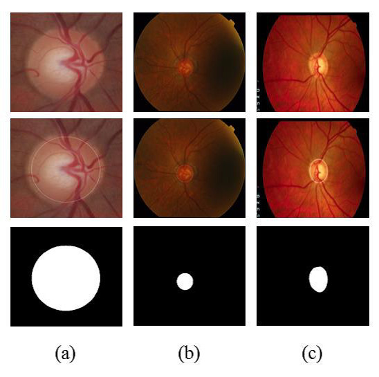
Figure 3 shows examples of segmentation process. Figure 3(a) shows an image of the RIM-ONE database along with the OD region, found by methodology and segmented region. Figures 3(b) and 3 (c) are similar to 3(a) but for DRISHTI-GS and DRIONS-DB databases, respectively.

Quantitative evaluation of the proposed segmentation method is presented in Section 5.

3.2 Feature Extraction

The extraction of attributes aims to describe the images according to the extracted features. These features are used for pattern recognition. Depending on the purpose of the problem, feature extraction can return different features to a same image [13]. In this work we used Gray-Level Co-occurrence Matrix (GLCM) to the extraction of texture features in different color models. ]]> GLCM is a technique used in texture analysis area, which was developed in the 70s by the researcher Robert M. Haralick [14]. It is a statistical method for feature extraction, which will be analyzed existing co-occurrences between pairs of pixels, in other words it is not examined each pixel individually but the pixel sets related through some pattern.

The GLCM is a square matrix that keeps informations of the relative intensities of the pixels in a image. It calculates the probabilities of co-occurrence of two gray levels i and j, given a certain distance (d) and an orientation () which can assume the values of 0^o, 45^o, 90^o and 135^o [15]. All information on the texture of an image will be contained in this matrix.

From the GLCM, Haralick set 14 significant features, and the number of features used in a particular problem varies in accordance with its specifications [14]. Use all these features is not always needed. Actually, can worsen the performance of the method instead of improving. After be observed and tested the features, five of them were selected: Contrast, Homogeneity, Correlation, Entropy and Energy.

The Contrast returns a measure between the intensity of a pixel and its neighbor. The comparison performed in all image pixels can be calculated from Equation 5.

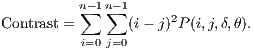(5)

The Homogeneity returns a value that represents the proximity of distribution of elements in relation to the diagonal of the matrix of co-occurrence of the gray levels. Its calculation is shown in Equation 6.

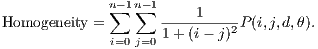(6)

The Correlation returns a measure of how correlated is a pixel with its neighbor. The comparison is made on all pixels of the image and is calculated by Equation 7.

(7)

where and represent the average for x and y directions, respectively, and represent the standard deviation. ]]> The Entropy measures the information contained in P, the degree of gray levels dispersion. Many null values represent little information. Its calculation is demonstrated in Equation 8.

(8)

The Energy returns the sum of elements elevated square in the matrix of co-occurrence of gray levels, where its calculation is shown in Equation 9.

(9)

In this context and based on some studies in the literature [11] and [12], this paper aims to extract the attributes of GLCM matrix in several colors bands of segmented images obtained in the previous section.

Each retinal image has been converted to color models: RGB (Red, Green and Blue), HSI (Hue, Saturation and Intensity) and L*u*v. Then GLCM matrix was calculated for all bands of these models. Contrast, homogeneity, correlation and energy were calculated for each matrix. After the description of the images, the classification of images was carried out in glaucomatous or not.

3.3 Classification

After the feature extraction it is not possible to predict if an image has Glaucoma or not, so it was necessary the classification step, where the attributes calculated in the previous step formed a vector, which served as input to the classifiers. At this step we used the classifiers MultiLayer Perceptron [16], Radial Basis Function (RBF) [17], Random Committee [18] and Random Forest [19]. Section 5 shows the results obtained for each one of these classifiers.

4 Performance Evaluation Metrics

In this section will be presented segmentation and classification evaluation metrics. ]]>

4.1 Segmentation Evaluation Metrics

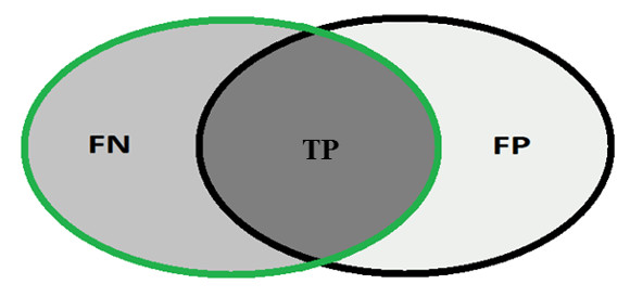
In order to calculate the measures of quantitative evaluation, we used the values of True Positive (TP), False Positive (FP) and False Negative (FN), as shown in Figure 4. These values are calculate using Equations 10, 11 and 12 respectively.

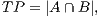(10)

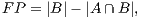(11)

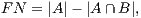(12)

where is the area of the ground truth and is the area of the region segmented by the algorithm. ]]> Using the values of TP, FP and FN we calculate Zijdenbos similarity index (ZSI) [20]. Equation 13 shows how to calculate the ZSI.

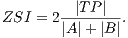(13)

We consider that a OD was segmented correctly if the ZSI between the ground truth and the segmented region is greater than a specific threshold. Finally, using this values we calculate the accuracy of the method.

4.1.1 Evaluation Metrics of Classifiers

Most analysis criteria of the results of a classification comes from a confusion matrix which indicates the number of correct and incorrect classifications for each class. A confusion matrix is created based on four values: True Positive (TP), number of images correctly classified as glaucomatous; False Positive (FP), number of images classified as healthy when actually they were glaucomatous; False Negative (FN), number of images classified as glaucomatous when actually they were healthy and True Negative (TN), number of images classified correctly as healthy.

From these amounts some statistics rates can be calculated to evaluate the performance of the classifiers. The rates of Precision, Recall, Accuracy and F-Measure (FM) are calculated respectively by Equations 14, 15, 16 and 17.

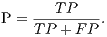(14)

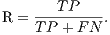(15)

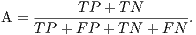(16)

(17)

Another measure used was the Kappa index, which has been recommended as an appropriate measure for fully represent the confusion matrix. It takes all the elements of the matrix into account instead of only those located on the main diagonal, which occurs when calculating the total accuracy of the classification [21]. ]]> The Kappa index is a concordance coefficient for nominal scales, which measures the relationship between the concordance and causality, beyond the expected disagreement [21]. The Kappa index can be found based on Equation  18.

(18)

In this case, ”observed” is the general value to the correct percentage, in other words, sum of the main diagonal of the matrix divided by the number of elements and ”expected” are the values calculated using the total of each row and each column of the matrix.

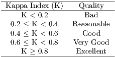
The categorization of the accuracy level of the result of classification, by the relation of Kappa index, can be seen in Table 1, as defined by Landis and Koch in 1977 [22].

---

Table 1: Accuracy level of a classification according to the value of the Kappa index.

---

5 Results

This section presents the results obtained for the segmentation and classification of images based on the proposed methodology. ]]> For the evaluation of segmentation were used three public image databases: RIM-ONE [23], DRISTHI-GS [24] and DRIONS-DB [25]. These bases have respectively 169, 50 and 110 pictures. Figures (a), (b) and (c) show examples of images from each of these three databases and their respective OD mask. An example of image of the RIM-ONE database and its OD marking is demonstrated in Figure  5 (a). Figure  5 (b) and (c) shows images of DRISTHI-GS and DRIONS-DB databases with their OD markings, respectively.

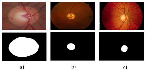
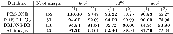
Table 2 shows the comparison between the results obtained by the proposed algorithm (1) and Rajaput et al.  [9] (2) algorithm. To determine the accuracy was used the ZSI measure (section 4.1) and the thresholds of 60, 70 and 80 %.

---

]]> Table 2: Comparison between accuracy obtained by the proposed algorithm and the Rajaput et al.

Based on the analysis of Table 2, it is clear that the proposed algorithm performed better in RIM-ONE and DRIONS-DB databases for all tested thresholds. The Rajaput et al. [9] method performed better in segmentation of the DRIONS DB database. Considering all the images, the proposed algorithm performed better, with an accuracy of over 92% using the threshold of 70%, which is the classic value used in the literature [20].

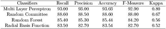
For evaluation of the classification results are used the measures of Precision, Recall, Accuracy, F-Measure and Kappa, seen in Section 4. The parameters used for classification were the standards of each classifier in WEKA (Waikato Environment for Knowledge Analysis) [26], and validation method used was the k-fold cross-validation (with k = 10). Table 3 shows the results of this classification.

---

Table 3: Results of the classification using the features extracted.

---

In Table 3, Multi Layer Perceptron classifier has obtained the best performance, with an accuracy of 93.03% and kappa of 0.8. According to Table 1, the MLP obtained a performance considered ”Excellent”. The Random Committee obtained a performance ”Very Good” and RBF and Random Forest obtained performance considered ”Good”. ]]> The results showed that the texture features are important in the detection of Glaucoma. The results of the classification are considered good according to Table 1, which presents the interpretation of Kappa index values.

6 Conclusion and Future Work

Digital image processing has become an area of study with great potential, which increasingly has contributed to society. In the health area, the digital image processing is being used in supporting diagnostic of diseases to be carried out effectively and cheaply.

This paper presented a methodology for automatic detection of the OD in digital images of fundus of eye. Then, from this region the texture features were extracted using the GLCM matrix in different color models. The evaluation of the detection of the OD was performed in three different image databases. The segmentation showed efficient results, accounting an accuracy greater than 83% when evaluated using a success rate requirement of 70%, which is the classical value found in the literature.

After the segmentation, the extraction of texture features of the images was performed. Then, it was carried out the classification of the retinal images in glaucomatous or not glaucomatous. Multi Layer Perceptron classifier obtained the best results with an accuracy of 93.03% and the Kappa index of 0.80.

As future work will be compared the results of the segmentation proposed in this work with the results obtained by classic algorithms of detection of the OD proposed in the literature. Another future work is to implement an automatic segmentation algorithm of excavation of the OD in order to calculate the CDR (Cup-to-Disc Ratio) that is the ratio between the excavation area and the OD area. The calculation of the CDR is widely used by doctors in supporting detection of Glaucoma.

References