, the minimal cardinality of the set of candidate species that the tested algorithms render as best matches is also presented in this research]]>
Combining Leaf Shape and Texture for Costa Rican Plant Species Identification
Carranza-Rojas, Jose Computer Engineering Department Costa Rica Institute of Technology jcarranza@itcr.ac.cr Mata-Montero, Erick Computer Engineering Department Costa Rica Institute of Technology emata@itcr.ac.cr
]]>
Abstract
In the last decade, research in Computer Vision has developed several algorithms to help botanists and non-experts to classify plants based on images of their leaves. LeafSnap is a mobile application that uses a multiscale curvature model of the leaf margin to classify leaf images into species. It has achieved high levels of accuracy on 184 tree species from Northeast US. We extend the research that led to the development of LeafSnap along two lines. First, LeafSnap’s underlying algorithms are applied to a set of 66 tree species from Costa Rica. Then, texture is used as an additional criterion to measure the level of improvement achieved in the automatic identification of Costa Rica tree species. A 25.6% improvement was achieved for a Costa Rican clean image dataset and 42.5% for a Costa Rican noisy image dataset. In both cases, our results show this increment as statistically significant. Further statistical analysis of visual noise impact, best algorithm combinations per species, and best value of , the minimal cardinality of the set of candidate species that the tested algorithms render as best matches is also presented in this research.
Abstract in Spanish: En la última década, la investigación en Visión por Computadora ha desarrollado algoritmos para ayudar a botánicos e inexpertos a clasificar plantas basándose en fotos de sus hojas. LeafSnap es una aplicación móvil que usa un modelo de curvatura con multi-escala del margen de la hoja para clasificar especies de plantas. Ha obtenido altos niveles de exactitud con 184 especies de árboles del noreste de Estados Unidos. Extendemos la investigación de LeafSnap en dos aristas. Primero, se aplican los algoritmos de LeafSnap en un set de datos de 66 especies de árboles de Costa Rica. Luego, la textura es usada como criterio adicional para medir el nivel de mejora en la detección automática de especies de árboles de Costa Rica. Una mejora de un 25.6% se logra con el set de datos limpio y un 42.5% para el set de datos sucio de Costa Rica. En ambos casos, los resultados muestran un incremento significativo en la exactitud del modelo. Además se presenta un análisis estadístico del impacto visual del ruido, las mejores combinaciones de algoritmos por especie, y el mejor valor de k, que es la cardinalidad mínima del set de especies candidatas que surgen como respuesta de identificación.
Keywords: Biodiversity Informatics, Computer Vision, Image Processing, Leaf Recognition Keywords in Spanish: Informática para la Biodiversidad, Visión por Computadora, Procesamiento de Imágenes, Reconocimiento con Hojas, Reconocimiento de Especies Received: 2015-10-31 Revised: 2016-03-23 Accepted: 2016-04-11 DOI: http://dx.doi.org/10.19153/cleiej.19.1.7
1 Introduction
]]>
Plant species identification is fundamental to conduct studies of biodiversity richness of a region, inventories, monitoring of populations of endangered plants and animals, climate change impact on forest coverage, bioliteracy, invasive species distribution modelling, payment for environmental services, and weed control, among many other major challenges for biodiversity conservation. Unfortunately, the traditional approach used by taxonomists to identify species is tedious, inefficient and error-prone [1]. In addition, it seriously limits public access to this knowledge and participation as, for instance, citizen scientists. In spite of enormous progress in the application of computer vision algorithms in other areas such as medical imaging, OCR, and biometrics [2], only recently have they been applied to identify organisms. In the last decade, research in Computer Vision has produced algorithms to help botanists and non-experts classify plants based on images of their leaves [3,4,5,6,7,8,9,10,11,12]. However only a few studies have resulted in efficient systems that are used by the general public, such as [13]. The most popular system to date is LeafSnap [13]. It is considered a state-of-the-art mobile leaf recognition application that uses an efficient multiscale curvature model to classify leaf images into species. LeafSnap was applied to 184 tree species from Northeast USA, resulting in a very high accuracy method for species recognition for that region. It has been downloaded by more than 1 million users [13]. LeafSnap has not been applied to identified trees from tropical countries such as Costa Rica. The challenge of recognizing tree species in biodiversity rich regions is expected to be considerably bigger.
Vein analysis is an important, discriminative element for species recognition that has been used in several studies such as [14,15,16,17,18]. According to Nelson Zamora, curator of the herbarium at the National Biodiversity Institute (INBio), venation is as important as the curvature of the margin of the leaf when classifying plant species in Costa Rica [19].
This paper focuses on studying the accuracy of a leaf recognition model based not only on the curvature of the leaf margin, but also on its texture (in which veins are visually very important). This is the first attempt to create such model for Costa Rican plant species.
The rest of this manuscript is organized as follows: Section 2 presents relevant related work. Section 3 and Section 4 cover methodological aspects and experiment design, respectively. Section 5 describes the results obtained. Section 6 presents conclusions and, finally, Section 7 summarizes future work.
2 Related Work
In LeafSnap [13] the authors create a leaf classification method based on unimodal curvature features and similarity search using k Nearest Neightbors (kNN). This method is tested against an image dataset from North American trees, using 184 species in total. Since their system requires images to have a uniform background, leaf segmentation works by estimating the foreground and background color distributions, and then classifying each pixel at a time into one of those two categories. A conversion to Hue Saturation Value (HSV) color domain is applied before using Expectation-Maximization (EM) [20] for the leaf segmentation. A 96.8% of accuracy is reported by the authors on their dataset with .
Researchers in [21] use Local Binary Patterns (LBP) features to classify medicinal and house plants from Indonesia. They extract LBP descriptors from different sample points and radius, calculate a histogram for each radius length feature set, and concatenate those histograms, similarly to Histogram of Curvature over Scale (HCoS) of LeafSnap [13]. As a classifier, a four layer Probabilistic Neural Network (PNN) is used. Their dataset consists of two subsets; one comprises 1,440 images of 30 species of tropical plants, and the other one has 300 images of 30 house plant species. The image background of the medicinal plants is uniform, while house plant images have non-uniform backgrounds. For medicinal plants the reported precision is 77% and for house plants 86.67%, revealing that using LBP for complex image backgrounds is a suitable technique.
Authors in [22] use Speeded Up Robust Features (SURF) to develop an Android application for mobile leaf recognition. For the species classification task, SURF features are extracted from the gray scale image of the leaf. The feature set is reduced to histograms in order to reduce dimensionality since the resulting SURF feature vector may be too big. The precision reported is 95.94% on the Flavia dataset [6], which consists of 3,621 leaf images of 32 species.
3 Methodology
This section describes how the leaf recognition process was set up. Section 3.1 describes the image datasets used. Section 3.2 summarizes the techniques used to segment each image into leaf and non-leaf pixels clusters. Section 3.3 presents several image enhancements conducted, such as cleaning up undesirable artifacts and elements, stem removal, clipping and resizing. Section 3.4 describes the feature extraction approach for both the curvature and texture model. Finally, Section 3.5 presents the species classification metrics and algorithms used in this research. ]]>
3.1 Image Datasets
An image dataset of leaves from Costa Rica was created from scratch. To our knowledge, no other suitable Costa Rican datasets existed before. The dataset has both clean and noisy images, in order to identify how the amount of noise affects the algorithms. All images were captured from mainly two places: La Sabana Park, located in San Jose, and INBiopark, located in Santo Domingo, Heredia. In most cases, images for both surfaces of each leaf were taken. The dataset includes endemic species of Costa Rica and threatened species according to [19]. The complete list of species in the dataset can be found in [23]. The dataset consists of the following two subsets:
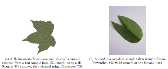
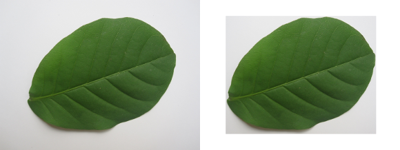
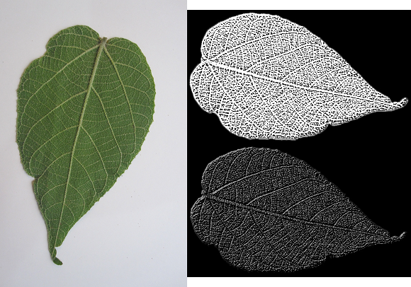
Clean Subset Fresh leaf images were captured during field trips to both La Sabana and INBiopark. If the leaves were not flat enough, a press was used to flatten them for 24 hours. A total of 1468 leaf images were scanned. The images have a white uniform background and a size of 2548x3300 pixels, scanned with 300 dpi in JPEG format. Photoshop CS6 was used to remove shadows, dust particles and other undesired artifacts from the background. Figure ?? shows a sample of a cleaned Costa Rican leaf image of this subset. The scanner used was an HP ScanJet 300.
Noisy Subset Fresh leaf images were captured during field trips to both La Sabana and INBiopark. No press was used to flatten them. A total of 2345 fresh leaf images were captured. This subset was captured against white uniform backgrounds (normally a sheet of paper). Each image has a 3000x4000 pixel resolution, in JPG format. No artifacts were removed manually. However as explained in Section 3.3 several automated image enhancements were performed both on the clean subset and the noisy subset. Figure ?? presents a noisy leaf image sample. The camera used is a Canon PowerShot SD780 IS.
Figure 1: Collected image samples
3.2 Image Leaf Segmentation
]]>
The first step to process the leaf image is to segment which pixels belong to a leaf and which do not. We used the same approach as LeafSnap by applying color-based segmentation.
3.2.1 HSV Color Domain
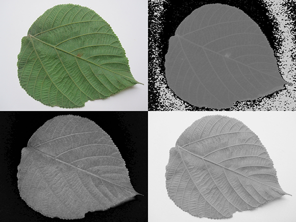
When segmenting with color it is imperative to use the right color domains in order to exclude undesired noise. [13] states how, in the HSV domain, Hue had a tendency to contain greenish shadows from the original leaf pictures. Saturation and Value however, had a tendency to be clean. So we also used those two color components for leaf segmentation. Figure 2 shows the noise present in the Hue channel, but also shows how Saturation and Value are cleaner. This was useful for posterior segmentation using Expectation-Maximization (EM). We used OpenCV [24] to convert the original images into the HSV domain. Then, by using NumPy [25] , we extracted the Saturation and Value components, which were fed to the Expectation-Maximization (EM) algorithm.
Figure 2: HSV decomposition of a leaf image
The top-left image shows the original sample. The top-right image shows the Hue channel of the image with noticeable noise. The bottom-left image shows the Saturation component and the bottom-right image shows the Value component
3.2.2 Expectation-Maximization (EM)
]]>
Once images were converted to HSV and the desired channels were extracted, we applied EM to the color domain in order to cluster the pixels into one of 2 possible groups: leaf and non-leaf groups [13]. Figure 3 shows several samples of the final segmentation after applying EM. As shown, EM segments the image into the leaf and non-leaf pixel groups by assigning a to the leaf pixels and a to the non-leaf pixels. This method also works well on both simple and compound leaves. It is important to highlight that we did not assign weights to each cluster manually as the work done by [13], because we wanted to leave the process as automatic as possible. In their work, they improve the segmentation of certain types of leaves, especially skinny ones, by manually assigning different weights to each cluster. Weights play a fundamental role into the segmentation process as reported in [26].
Figure 3: Segmented Samples
After applying EM to different Costa Rican species
Training Algorithm 1 describes the process to train the EM algorithm. We used OpenCV’s implementation of EM. First we stacked all the pixels of the image matrix into a single vector. Then we trained the model using a diagonal matrix as a co-variance matrix, and we assigned two clusters to it, which internally were translated into two Gaussian Distributions, one for the leaf cluster and one for the non-leaf cluster. Once trained, we returned the EM object.
]]>
Algorithm 1: EM Training
for allin imagedo for allin pixelRowdo endfor endfor ]]>
return
Pixel Prediction Algorithm 2 explains how the owning cluster of a single pixel of the image was predicted. Once the EM object was trained, the OpenCV’s implementation allowed to compute the probabilities of the pixel belonging to each cluster. However, for more efficiency, we created a dictionary containing each unique pair as key, and the cluster as value. If the key was not found in the dictionary, we then proceeded to predict the probabilities for each cluster, added the key and cluster to the dictionary, and returned the associated cluster with the biggest probability.
After segmentation of the leaf using EM, some extra work was needed to clean up several false positives areas. We followed the process of LeafSnap [13]. First of all, each image was clipped to the internal leaf size provided by the segmentation. Then the image was resized to a common leaf area, followed by a heuristic applied to delete undesired objects. Finally, the stem was deleted since it added noise to the model of curvature (not that much to the texture model).
3.3.1 Clipping
Before extracting features, a clipping phase was needed in order to resize the region where the leaf was present to a common size. The clipping algorithm was trivial to implement once the contours were calculated using OpenCV. As shown in Algorithm 3, the minimum and maximum coordinates were calculated for all contour and components, followed by a cut of the leaf image matrix to those resulting minimum and maximum coordinates. The was used to allow posterior algorithms ignore false positives regions that intersect the border. The results of the Clipping phase can be seen in Figure 4.
]]>
Algorithm 3: Clipping Leaf Portion of the Image
]]>
Figure 4: Clipping of a Coccoloba floribunda sample
The left image is the original leaf image, and the right one is clipped to the leaf size
3.3.2 Resizing Leaf Area
Once the leaf area had been clipped, a resize was applied in order to standardize the leaf areas inside all images. If not, the model of curvature would be affected negatively since the amount of contour pixels varied significantly [13]. Our implementation of the resize was applied to the whole clipped image. Images may end up having different sizes, but the internal leaf areas were the same or almost the same. Algorithm 4 shows how a new width and height were obtained by calculating the ratio between the current leaf area, the desired new leaf area, and the current height and width of the image. Finally, OpenCV was used to resize the clipped image to a constant leaf size of pixels. This number was used empirically based on LeafSnap’s original dataset resolution and the internal regions associated with leaf pixels. This approach means that the absolute measures of leafs are lost.
Algorithm 4: Common Leaf Area Resize
]]>
return
3.3.3 Deleting Undesired Objects
Even when uniform background images were used, initial segmentation turned out not to be enough when the image contained undesired objects, such as dust, shadows, among others. [13] attempted to delete these noisy objects by using the same heuristic we implemented as shown in Algorithm 5. By using Scikit-learn [27] we calculated the connected components of the segmented image. We deleted the ”small” components by area (in pixels). Small components were normally dust, small bugs or pieces of leaves, among other things. Once all small components were deleted, if the remaining was only one then we took that to be the leaf. If more than one component remained, then we calculated for each remaining component how many pixels had intersections with the image margin. We then deleted the component with the biggest number of intersections. The thinking behind this is to get rid of components that were not centered on the image, which tend to be non-leaf objects. Finally, the component with the biggest area from the remaining components was taken as the leaf.
]]>
Algorithm 5: Deleting Undesired Objects Heuristic
ifthen return endif ]]>
for allindo endfor return
3.3.4 Deleting the stem
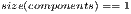
We followed the approach for stem deletion described in [13]. If the stem was left intact, it would add noise to the model of curvature, given all the possible sizes the stem may take. Algorithm 7 shows the procedure. First, a Top Hat transformation was applied to the segmented image in order to leave only possible stem regions, as shown in Figure 5. Then all connected components were calculated from the Top Hat transformed image, and also their quantity. Then we looped over all the components, deleting every single one from the original segmentation and recalculating the new number of connected components. If the original number of recalculated connected components did not change upon deletion, that meant the current component was a good stem candidate (heuristically, a stem does not affect how many original connected components there are). Once all stem candidates were calculated, the one with the biggest area and largest aspect ratio was chosen to be the stem, as described in Algorithm 6.
]]>
Algorithm 6: Calculate Aspect Ratio Combined with Area
return
Algorithm 7: Deleting the Stem
]]>
for allindo ifthen endif endfor ]]>
Figure 5: Top Hat Transformation applied to a segmented compound leaf image to detect the stem of the leaf
3.4 Leaf Feature Extraction
Feature extraction was designed and implemented considering three main design goals:
Efficiency: algorithms should be fast enough to support future mobile apps.
Rotation invariance: the leaf may be rotated by any angle within the image.
Leaf Size Invariance: datasets contain different sizes of leaves and users can capture images independently of the relative size of leaves.
]]>
Two different feature sets were calculated. The first one captures information about the contour of the leaf, while the second one captures information about its texture. Section 3.4.1 describes how we implemented Histogram of Curvature over Scale (HCoS) [13] to extract contour information. Section 3.4.2 describes how we implemented Local Binary Pattern Variance (LBPV) to extract texture information. Both models generate histograms that are suitable for distance metric calculations.
3.4.1 Extracting contour information (HCoS)
The model of curvature used by LeafSnap comprises several steps. Previously explained segmentation and post-processing resulted in a mask of leaf and non-leaf pixels. The non-leaf pixels have values of , and the leaf pixels have values of . First, the different contour pixels were found, then 25 different masks with disk shapes were applied on top of each contour point, providing both an area of the intersection and an arc length. Then all calculations at each scale were turned into a histogram, resulting in 25 different histograms per image, one per scale. Finally, the 25 resulting histograms were concatenated, conforming the HCoS.
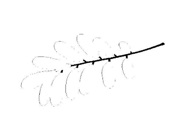
Contours On a binary image (resulted from the previous segmentation), the OpenCV implementation of contour finding worked very well, based on the original algorithm of [28] for contour finding. The algorithm generated in a vector of pairs that represent the coordinates where a contour pixel was found. A contour pixel can be defined as a pixel which is surrounded by at least another pixel with the opposite color of it. Figure 6 shows in red the contour pixels detected in the original image, calculated from the segmented mask. Notice how shadows affect the contour algorithm, since they were not segmented perfectly.
The disks used are actually matrices of ’s and ’s. They were applied as masks over specific parts of the segmented leaf image (mostly contour points). The idea was to count how many pixels intersected the segmented image and each disk mask. We created two different types of disks. The first type is filled up with ’s, as shown in Figure 7. It is used to measure the area of intersection. The second type is more like a ring, where ’s are present only in the circumference of the disk (see Figure 7). It is used to determine the arc’s length of the intersection of the disk with the leaf, at a given contour point.
Figure 7: Various discrete disks
Once all disks were created for both area and arc length versions, we applied them to each pixel of the contour vector, as shown by Algorithm 8. ]]>
Algorithm 8: Area and Arc Length Vector Calculation
for allof the contour vectordo for alltodo centerat current contour ]]>
endfor endfor
Figure 8 shows how one specific area disk was applied to the segmented image, for an specific scale (radius= in this case), at a given contour pixel. The gray area shows the intersection of pixels with the leaf segmentation. This procedure was then repeated over all the pixels from the contour vector in the same way.
]]>
Figure 8: Area disk applied
to a Croton niveus sample at an specific pixel of the contour, with radius=
Histograms Using NumPy at each scale, a histogram was created from all the values generated from all contour pixels, as described by Algorithm 8. We used histograms of 21 bins, as [13] did. This means a total of 25 different histograms were created, each with 21 bins, per image. At each scale, each histogram was normalized to unit length. Then, all histograms were concatenated together (both the 25 for area and 25 for arc length), generating what [13] describes as the Histogram of Curvature over Scale (HCoS).
3.4.2 Extracting texture information (Local Binary Pattern Variance (LBPV))
We aimed at improving the model of curvature by adding texture analysis. We used a Local Binary Pattern Variance (LBPV) implementation called Mahotas [30] that is invariant to rotation, multiscale, and efficient. This implementation of LBPV is based on the algorithm of [31] and makes use of NumPy libraries to represent the image and the resulting histograms. It works on gray images, so we used OpenCV to convert the Red Green Blue (RGB) images to gray scale images. The LBPV approach detects micro structures such as lines, spots, flat areas, and edges [31]. This is useful to detect patterns of the veins, areas between them, reflections, and even roughness. Figure 9 shows what two different LBPV implementations look like. The upper image shows a (R2P16) implementation, and the one below shows a (R1P8) pixel implementation. The different variants of the LBPV used are shown in Table 1. In some cases we concatenated two histograms of different scales such as R1P8 & R2P16. It is important to note that we did not use the variant which samples 24 pixels, since it generated too large histograms. We did, however, run some tests in which we noticed the 24 pixels variation didn’t add more accuracy, so we decided to ignore this method.
Table 1: Variants of LBPV
]]>
Figure 9: LBPV patterns of a Croton draco sample. The upper image corresponds to a (R2P16) and the lower one to a (R1P8) pattern
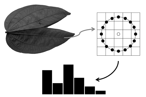
Just like the HCoS, LBPV generates histograms that can be used for similarity search. Several histograms were generated at different radius sizes and different circumference pixel sampling, in order to validate which combinations provided the best results. The Mahotas implementation returned a histogram of the feature counts, where position corresponds the count of pixels in the leaf texture that had code . Also, given that the implementation is a LBPV, non-uniform codes are not used. Thus, the bin number is the feature, not just the binary code [30]. Figure 10 describes at a very high level how the process of extracting the local patterns histograms works. First, the image is converted to a gray scale image. Then, for each pixel inside the segmented leaf area, we calculated the local pattern with different radius and circumference using the mahotas implementation. Finally, each pattern was assigned to a bucket in the resulting histogram. Each pixel has a number assigned to it corresponding to a pattern, and the histogram was created using all those numbers from the segmented leaf pixels.
]]>
Figure 10: Process of extracting LBPV
3.5 Species Classification based on Leaf Images
Once all histograms were ready and normalized, a machine learning algorithm was used to classify unseen images into species. We implemented the same classification scheme used by LeafSnap. The following paragraphs describe how k Nearest Neightbors (kNN) was implemented.
Scikit-learn’s kNN implementation was used for leaf species classification. This process was fed with previously generated histograms from both the model of curvature using HCoS and the texture model using LBPV. Additional code was created to take into consideration only the first matching species, not the first images, as shown by Algorithm 9. The difference resides in taking into account only the best matching image per species, until completing the first species [13].
Algorithm 9: k Species Ranking
]]>
while eachdo if notinthen endif endwhile
We used in order to measure how different algorithms behaved as the value of increased.
3.6 Distance Metric - Histogram Intersection
We tested the basic Euclidean distance to measure similarity between histograms, however the results were not encouraging. We implemented the histogram intersection shown on Equation 1, where is the histogram intersection between a histograms and of same size, is the number of bins, and and are each a bin in histograms and , respectively. This distance metric is also normalized to unit length.
(1)
]]>
3.7 Accuracy
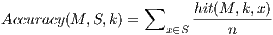
Let be an identification experiment that consists of a model , a set that contains images of leaves of (not necessarily different) unknown tree species to be identified, and an integer value , . We define as a boolean function that indicates if model generates a ranking in which one of the top candidate species is a correct identification of sample . Equation 2 formally defines .
(2)
4 Experiments
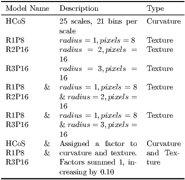
Several model variations were used in the experiments (see Table 2).
1.
Our implementation of LeafSnap’s model of curvature HCoS.
2.
Several scales of the texture model based on LBPV.
3.
The combination of HCoS and the best LBPV variant, which according to our tests was R1P8 & R3P16. This combination was further disaggregated by assigning different weights to HCoS and the texture model.
Table 2: Models used in the experiments including curvature, variants of texture model, and combination of both
]]>
One Versus All One approach to test a model is to partition a dataset into two datasets: one for training and one for testing. Another approach is to use One versus All, that is, each image in a dataset with elements is considered a test image and the remaining images the training subset. We used both approaches as explained at the end of this section.
Combining Curvature and Texture When combining two different models, we faced the issue of having different scales in the resulting ranking of each model. This was resolved by normalizing the rankings to unit length.
After normalizing the rankings (one per combined algorithm), we assigned a factor to each combined model in order to rank the predicted species into a single ranking. This factor sums in total. However we varied the factor associated with each model to see the behavior across different combinations. We used factors of (0.10, 0.90), (0.20, 0.80), (0.30, 0.70), (0.40, 0.60), (0.50, 0.50), (0.60, 0.40), (0.70, 0.30), (0.80, 0.20), (0.90, 0.10). For example, means we gave the same level of importance to each model on that combination. Algorithm 10 describes how the merge between two methods was achieved.
Algorithm 10: Combining Two Rankings
]]>
for allindo for allindo endfor endfor
4.1 Texture and Curvature Model Experiments
We ran all models described in Table 2, with , and the following data sets: Costa Rica clean subset (One versus All, ), Costa Rica noisy subset (One versus All, ), and Costa Rica complete data set (training set with all clean images and testing set with all noisy images). In each experiment, was calculated for the corresponding dataset . In addition, for model HCoS & R1P8 & R3P16, Algorithm 10 was used to comprehensively consider different weight combinations for HCoS and the texture model. Table 5 summarizes the results obtained. ]]>
4.2 Processing Times
To understand the duration of the recognition process, we measured the recognition time for all images from both Costa Rican noisy and clean subsets, as if a back-end received images from a mobile app. The measured time includes image loading, segmentation, stem deletion, normalization, curvature calculations, texture calculations, and similarity search. It does not include network related times. We used a MacBook Pro with an Intel Core i7, GHz, and GBs on RAM.
4.3 Statistical Analysis For Noise Affectation, Best Algorithms per Species, and best value
Using the clean and noisy datasets, we calculated a General Linear Model (GLM) per species over a total of 65 species. We aimed at discovering the following:
What is the minimum value of that provides results statistically equivalent to those obtained when for each species? Obviously, accuracy increases as the value of increases. However, for practical reasons, we would like to test if there is a threshold value after which accuracy remains statistically equivalent to using . For example, in a mobile app users would appreciate if the number of best ranked species is not the maximum value 10, but a smaller number.
What is the best algorithm or combination of algorithms for each species? For this we used five different algorithms: R1P8 & R3P16 (texture alone), HCoS and R1P8 & R3P16, HCoS and R1P8 & R3P16, HCoS and R1P8 & R3P16 and HCoS (curvature alone). This also includes creating clusters of species based on their most significant algorithms, and understanding the clusters with more species and best accuracies.
Does noise decrease the accuracy level obtained per species? Can we find some species that are not affected by noise in the data?
To achieve this, we calculated a GLM per species to detect significance of noise, algorithm used and value of . We used a confidence level of . Once each GLM was calculated and each main effect significance known and proven, we calculated if all levels within each factor were statistically equivalent. We are actually trying to find the levels that are significantly different, for all three factors.. We used a Tukey statistical test for each factor. Table 3 shows the different factors and levels used during this experiment.
Table 3: Factors and levels for GLM per species
]]>
4.4 Statistical Analysis of Best Algorithms for
Because has become an informal benchmarking value in other research [13], it is important to discover what algorithms got the best accuracy when . For this experiment, we ran a Binary Logistic Regression and optimized it, thus maximizing the probability of a successful identification. Based on the resulting regression model, we calculated the two best algorithms for both noisy and clean factors, and , per species.
5 Results
5.1 Comparison with Others Studies
In order to set a baseline, several other studies have used the Flavia dataset for their research [6]. Table 4 shows the comparison of these studies and our approaches. Some studies do not report accuracy but precision only. The best accuracy of our work was achieved, on this dataset, by adding 0.5 HCoS and 0.5 R1P8 & R3P1 with for a 0.991. We also attempted to use texture only, which shows to be very extremely accurate with up to 0.98. This dataset has been, however, artificially cleaned, so other studies should be evaluated on more complex datasets.
Table 4: Other studies comparison of obtained results on the Flavia dataset
5.2 Texture and Curvature Model Experiments
]]>
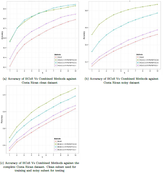
Clean Subset As shown in Table 5, the best results were obtained when and the model is HCoS and R1P8 & R3P16. The resulting accuracy is , in contrast with the accuracy of HCoS which is . Notice however that HCoS and R1P8 & R3P16 is also the best for all values of . For , HCoS and R1P8 & R3P16 and HCoS and R1P8 & R3P16 have very similar levels of accuracy. Figure 11 more clearly depicts these comparisons.
Noisy Subset Figure 11 clearly shows that HCoS and R1P8 & R3P16 has the best accuracy for all values of . In addition, the level of accuracy improvement with respect to HCoS is considerably larger, ranging from when to when as shown in Table 7.
Complete Dataset As Figure 11 shows, the level of accuracy is considerably lower for all models, as compared to the previous two experiments. Even the best model achieves levels of accuracy in a poor range.
Table 5: Accuracy obtained when combining curvature and texture over the clean subset, the noisy subset, and the complete Costa Rican dataset
]]>
Figure 11: Comparison of HCoS and Combinations
Discussion These experiments show how, in general, the combination of HCoS and LBPV consistently increases the accuracy of HCoS alone. Accuracy declines as the combination factor assigned to curvature reaches . Overall, the best combination seems to be HCoS and LBPV. It is also important to notice how the accuracy is sensitive to the quality of the dataset. The clean subset has a tendency to improve the recognition accuracy, in contrast with the noisy subset. This reflects the importance of good pre-processing and good segmentation. Shadows, dust, and other artifacts affect the final accuracy results.
5.3 Measuring Significance of the Accuracy Increase
As shown in the previous section there is an increase in accuracy when texture is added to our implementation HCoS. This, however, may not be statistically significant. We proceeded then to apply a Statistical Proportion Test for Two Samples. Our null hypothesis is that the accuracy of the implementation of HCoS equals the ones obtained by combining curvature and texture. In contrast, our alternative hypothesis is that the accuracy of the implementation of HCoS is less than the combinations.
Proportion Tests on the Clean Subset Table 6 shows the results obtained for all the proportion tests for the clean subset. Most combinations of HCoS and R1P8 & R3P16 for resulted in very low p-Values, which reject . However a few accuracy increases from HCoS and R1P8 & R3P16 did fail the test. This means that, as the weight increases for HCoS, it starts getting non-significant accuracy increases, which makes sense since it is almost equal to HCoS alone.
Proportion Tests on the Noisy Subset Table 7 shows the results obtained for all the proportion tests for the noisy subset. All combinations of HCoS and R1P8 & R3P16 resulted in very low p-Values, which reject .
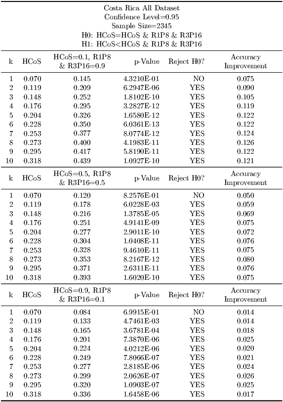
Proportion Tests on the Complete Dataset Table 8 shows the results obtained for all the proportion tests on the complete dataset of leaf images from Costa Rica. Almost every single test rejected . For the results are not significant. ]]>
In all Proportion Tests, by adding texture with a bigger factor the model improves significantly the accuracy. As the factor assigned to texture declines, the improvement becomes statistically insignificant.
Table 6: Proportion Test results over the Costa Rican Clean Subset
Table 7: Proportion Test results over the Costa Rican Noisy Subset
]]>
Table 8: Proportion Test results over the Costa Rican Complete Dataset
5.4 Processing Time
As shown in Figure 12, times range from to seconds. However, the median of the elapsed time is seconds for the clean subset and seconds for the noisy subset. These are suitable times even for mobile applications that use the developed back-end.
]]>
Figure 12: Box Plot of leaf image recognition times simulating a mobile app back-end, for Costa Rican noisy and clean subsets
5.5 Statistical Analysis of Noise Affectation, Best Algorithms per Species, and best value of
Table 9 shows the results of each GLM per species. Each species has the accuracy maximum, mean and median. Also, a cluster has been assigned regarding the best algorithms resulted from the Tukey test per species. Table 10 depicts the algorithms in each cluster for reference. Additionally, column ”Best Without Noise” indicates if noise does affect or not the accuracy for each species. Finally, column ”” indicates the threshold value per species. As indicated before, any will be slightly better, but this is not statistically significant.
Table 9: Per Species Table with Accuracy Mean, Maximum, Best Algorithms, Affectation by Noise and
]]>
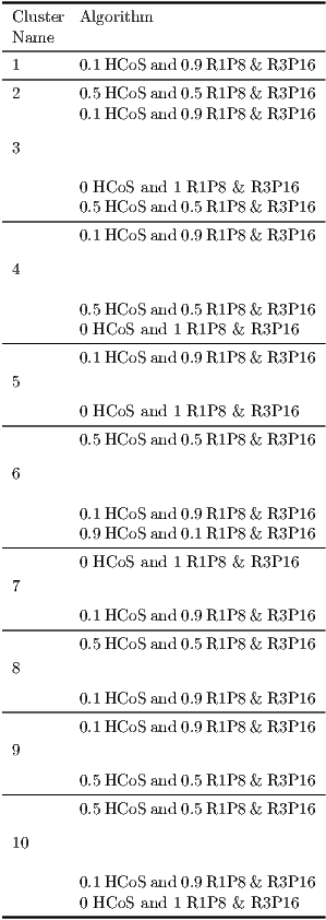
Table 10: Cluster definition and most significant Algorithms per Cluster
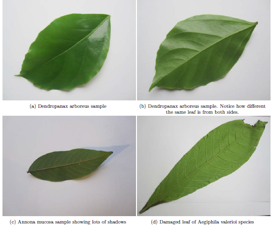
Noise Affectation. As Table 9 shows, most species are affected negatively by noise in the data. However, four species do show no significant difference between noisy and clean data. Blackea maurafernandesiana, Brosimumalicastrum, Hura crepitans, and Picramnia antidesma seem to be fairly resilient to noise with these algorithms. Table 9 shows some species which got low accuracy values at the bottom. Annona mucosa and Dendropanax arboreus got a median accuracy of 0.48, and Aegiphila valerioi of 0.45. Figure 13 shows 4 images of these 3 species. We suspect the reasons behind the low accuracy for these species are the shadows present inside the leaf and outside, against the paper sheet. Also it can be noticed some leaves also have physical damage. Dendropanax arboreus in Figure 13 also shows how different both sides of the same species are, suggesting we need to separate the dataset in both sides of the leaves.
Figure 13: Leaf samples of species with low accuracy
]]>
Value of threshold. The best is achieved by species Muntingia calabura, with . Bauhinia purpurea also shows a low value of . Eugenia hiraeifolia, Genipa americana, Hura crepitans, Quercus corrugata and Urera caracasana have . Overall, 13 species show a value, while 20 species have , and the rest result in . As is lower, then the potential maximum accuracy for that species tends to be very high.
Best Algorithms per species. Several clusters were identified based on algorithms that showed the best accuracy per species. Table 10 shows the list of clusters. Each cluster contains one to three algorithms that had the same statistical significance during our experiments per species. We have in total 10 clusters based on the best, second best and third best algorithm per species. Table 9 shows that most of the species belong to clusters that had the combination of HCoS and R1P8 & R3P16. Some also have R1P8 & R3P16 which is texture alone without curvature.
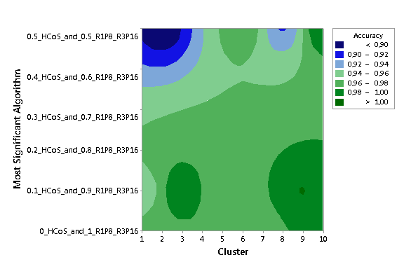
Figure 14 shows the accuracy distribution across the 10 clusters formed after carrying out Tukey tests on the different algorithms. The best algorithms have the biggest factor for texture. Cluster 3, Cluster 8 and Cluster 10, have as the best algorithm the combination HCoS and R1P8 & R3P16, and have the second best accuracy across all species. The very best cluster is Cluster 9, reaching an Accuracy of .
Figure 14: Accuracy distribution across different clusters found on the species
]]>
Figure 15 shows the distribution of species count per cluster. The cluster with the most species is Cluster 5, with more than 25 species. This cluster, as shown in Table 10, contains two best algorithms: HCoS and R1P8 & R3P16 combination, and HCoS and R1P8 & R3P16 combination. This means both of them are statistically equivalent for these species.
Figure 15: Species count distribution across different clusters
5.6 Statistical Analysis of Best Algorithms for
Best Algorithms forand noisy dataset. Table 11 shows what algorithms maximize the probability of a good identification, given that and the noisy dataset is used. Most algorithms are combinations, from pure texture, to a HCoS and R1P8 & R3P16 combination. No combination gets near a pure curvature algorithm. Similar results are noted in Figure 16 where the best probabilities are around the HCoS and R1P8 & R3P16 combination. In general the distribution is very homogenous.
]]>
Figure 16: Distribution of Probability of successful identification with noisy data and
Best Algorithms forand clean dataset. Table 12 shows what algorithms maximize the probability of a good identification, given that and the clean dataset is used. In this case the best algorithms per species are more spread across most combinations. This is due the lack of noise in the data and the lesser affectation of the curvature algorithms. This, compared with the data of Table 11 confirms how texture seems to be more robust with noise. Figure 17 shows the distribution of probabilities of a good identification per algorithm. On clean data it seems the biggest probabilities are near the center with combinations around the HCoS and R1P8 & R3P16 combination.
Figure 17: Distribution of Probability of successful identification with clean data and
]]>
Table 11: Algorithms that maximize the probability of a good identification for all species on noisy data, with a fixed
Table 12: Algorithms that maximize the probability of a good identification for all species on clean data, with a fixed
]]>
6 Conclusions
The addition of texture increases significantly the accuracy of our implementation of the HCoS. When comparing HCoS versus the combination of HCoS and R1P8 & R3P16, for the Costa Rican clean subset, the improvement ranges from to , depending on the value of . Similarly, with the noisy subset, the improvement ranges from to . These improvements were proved to be statistically significant in our experiments.
The complete dataset experiments demonstrated that poor accuracy levels are achieved when noisy images are classified against clean images. We speculate that this is due to the many enhancements that leaf images underwent before being added to the clean dataset. First, leaves were pressed for 24 hours in order to flatten them and thus minimize the presence of shadows. Secondly, Photoshop was used to manually remove artifacts. Finally, image enhancement algorithms (e.g., stem removal) were applied. This result has important implications if a mobile application is developed, given that users will take noisy pictures. As a result we are left with two alternatives. The first one is to use a noisy dataset to train the classifier. Alternatively a clean dataset could be used but user images would need to undergo further automated image enhancements comparable to those performed manually with Photoshop.
Experiments for individual species provided some interesting results. Concerning minimal values of , i.e., the size of the set of candidates that are considered best possibilities in an identification process, good levels of accuracy were obtained for in 63% of the species. Working with noisy images had a negative effect on levels of accuracy on 61 out of 65 species studied, as compared to clean images and a clean dataset. Finally, texture also stands out in most individual cases as the determining factor for high accuracy levels as compared to leaf shape.
Our statistical analysis of best algorithms for did not render a clear winner but highlighted that the best combination of algorithms should use weigths smaller than 0.2 to HCoS.
7 Future Work
A natural next step in this research is to develop a mobile app that uses the georeference of photographs of leaves as an additional criterion to classify species. Most modern mobile phones already include excellent cameras and provide the option of automatically georeferencing any picture taken with these cameras. In addition to the reference image dataset such as the one developed for this research, maps of potential distribution of species of Costa Rican trees would be needed. Atta, a comprehensive and fully georeferenced database of thousands of species of organisms from Costa Rica developed by the National Biodiversity Institute (INBio) www.inbio.ac.cr and GBIF’s database 1 are excellent foundations to generate these potential distribution maps of species. In addition to curvature, texture, and georeferencing as discriminating factors, morphological measures of leaves are also frequently used by specialists to identify plant species. Some of these measures are: aspect ratio, which is the ratio of horizontal width to vertical length; form coefficient, which is a numerical value that grades the leaf shape as between circular (shortest perimeter for a given area) and filliform (longest perimeter for a given area); and blade and petiole length. Algorithms to calculate these measures have already been developed (e.g., WinFOLIA). However, they have not been integrated in computer vision systems for automatic identification of plant species.
A crowd sourcing approach could be a very efficient way to increase the size of the image dataset that currently comprises 66 plant species from Costa Rica. In addition, crowdsourcing could also be used to clean noisy pictures as a citizen science project.
Finally, the individual contribution of texture features such as venation, porosity, and reflection in characterizing a plant species has not been formally established. A more elaborate analysis of the leaf texture that disaggregates it into a separate layer for each these features would help understand and quantify their individual contribution.
Acknowledgement
To the National Biodiversity Institute of Costa Rica (INBio) and Nelson Zamora for their help with the leaf sample recollection and expert feedback during this research. ]]>
References
[1]M. R. de Carvalho, F. A. Bockmann, D. S. Amorim, C. R. F. Brandão, M. de Vivo, J. L. de Figueiredo, H. A. Britski, M. C. de Pinna, N. A. Menezes, F. P. Marques, N. Papavero, E. M. Cancello, J. V. Crisci, J. D. McEachran, R. C. Schelly, J. G. Lundberg, A. C. Gill, R. Britz, Q. D. Wheeler, M. L. Stiassny, L. R. Parenti, L. M. Page, W. C. Wheeler, J. Faivovich, R. P. Vari, L. Grande, C. J. Humphries, R. DeSalle, M. C. Ebach, and G. J. Nelson, “Taxonomic impediment or impediment to taxonomy? a commentary on systematics and the cybertaxonomic-automation paradigm,” Evolutionary Biology, vol. 34, no. 3-4, pp. 140–143, 2007. [Online]. Available: http://dx.doi.org/10.1007/s11692-007-9011-6
[2]A. Andreopoulos and J. K. Tsotsos, “50 years of object recognition: Directions forward.” Computer Vision and Image Understanding, vol. 117, no. 8, pp. 827–891, 2013. [Online]. Available: http://dx.doi.org/10.1016/j.cviu.2013.04.005
[3]L. R.D and V. S, “Plant classification using leaf recognition,” in Proceedings of the 22nd AnnualSymposium of the Pattern Recognition Association of South Africa, November 2011, pp. 91–95.
[4]M. S. K. M. Z. Rashad, B.S.el-Desouky, “Plants images classification based on textural features using combined classifier,” International Journal of Computer Science and Information Technology, vol. 3, no. 4, 2011.
[5]A. Bhardwaj, M. Kaur, and A. Kumar, “Recognition of plants by leaf image using moment invariant and texture analysis,” International Journal of Innovationand Applied Studies, vol. 3, no. 1, pp. 237–248, 2013. [Online]. Available: http://www.ijias.issr-journals.org/abstract.php?article=IJIAS-13-087-01
[6]S. Wu, F. Bao, E. Xu, Y.-X. Wang, Y.-F. Chang, and Q.-L. Xiang, “A leaf recognition algorithm for plant classification using probabilistic neural network,” in Signal Processing and InformationTechnology, 2007 IEEE International Symposium on, Dec 2007, pp. 11–16. [Online]. Available: http://dx.doi.org/10.1109/ISSPIT.2007.4458016
[7]T. Beghin, J. Cope, P. Remagnino, and S. Barman, “Shape and texture based plant leaf classification,” in Advanced Concepts for Intelligent Vision Systems, ser. Lecture Notes in Computer Science, J. Blanc-Talon, D. Bone, W. Philips, D. Popescu, and P. Scheunders, Eds. Springer Berlin Heidelberg, 2010, vol. 6475, pp. 345–353. [Online]. Available: http://dx.doi.org/10.1007/978-3-642-17691-3\_32
]]>
[8]D. Wijesingha and F. Marikar, “Automatic detection system for the identification of plants using herbarium specimen images,” Tropical Agricultural Research, vol. 23, no. 1, 2012. [Online]. Available: http://www.sljol.info/index.php/TAR/article/view/4630
[9]C. H. Arun, W. R. S. Emmanuel, and D. C. Durairaj, “Texture feature extraction for identification of medicinal plants and comparison of different classifiers,” International Journal of ComputerApplications, vol. 62, no. 12, January 2013.
[10]N. Aggarwal and R. K. Agrawal, “First and second order statistics features for classification of magnetic resonance brain images,” Journal of Signal and Information Processing, vol. 3, no. 2, pp. 146–153, 2012. [Online]. Available: http://dx.doi.org/10.4236/jsip.2012.32019
[11]Y. Herdiyeni and M. Santoni, “Combination of morphological, local binary pattern variance and color moments features for indonesian medicinal plants identification,” in Advanced Computer Scienceand Information Systems (ICACSIS), 2012 International Conference, Dec 2012, pp. 255–259. [Online]. Available: http://dx.doi.org/10.5120/10129-4920
[12]A. Kadir, L. E. Nugroho, A. Susanto, and P. I. Santosa, “Leaf classification using shape, color, and texture features,” International Journal of Computer Trends and Technology, 2011. [Online]. Available: http://arxiv.org/pdf/1401.4447.pdf
[13]N. Kumar, P. Belhumeur, A. Biswas, D. Jacobs, W. Kress, I. Lopez, and J. Soares, “Leafsnap: A computer vision system for automatic plant species identification,” in Computer Vision -ECCV 2012, ser. Lecture Notes in Computer Science, A. Fitzgibbon, S. Lazebnik, P. Perona, Y. Sato, and C. Schmid, Eds. Springer Berlin Heidelberg, 2012, pp. 502–516. [Online]. Available: http://dx.doi.org/10.1007/978-3-642-33709-3\_36
[14]J. Clarke, S. Barman, P. Remagnino, K. Bailey, D. Kirkup, S. Mayo, and P. Wilkin, “Venation pattern analysis of leaf images,” in Proceedings of the Second International Conference on Advancesin Visual Computing - Volume Part II, ser. ISVC’06. Berlin, Heidelberg: Springer-Verlag, 2006, pp. 427–436. [Online]. Available: http://dx.doi.org/10.1007/11919629\_44
[15]M. G. Larese, R. Namías, R. M. Craviotto, M. R. Arango, C. Gallo, and P. M. Granitto, “Automatic classification of legumes using leaf vein image features,” Pattern Recogn., vol. 47, no. 1, pp. 158–168, Jan. 2014. [Online]. Available: http://dx.doi.org/10.1016/j.patcog.2013.06.012
[16]K.-B. Lee, K.-W. Chung, and K.-S. Hong, “An implementation of leaf recognition system based on leaf contour and centroid for plant classification,” in Ubiquitous Information Technologiesand Applications, ser. Lecture Notes in Electrical Engineering, Y.-H. Han, D.-S. Park, W. Jia, and S.-S. Yeo, Eds. Springer Netherlands, 2013, vol. 214, pp. 109–116. [Online]. Available: http://dx.doi.org/10.1007/978-94-007-5857-5\_12
[17]K.-B. Lee and K.-S. Hong, “An implementation of leaf recognition system using leaf vein and shape,” International Journal of Bio-Science and Bio-Technology, pp. 57–66, Apr 2013.
]]>
[18]Y. Li, Z. Chi, and D. Feng, “Leaf vein extraction using independent component analysis,” in Systems, Man and Cybernetics, 2006. SMC ’06. IEEE International Conference on, vol. 5, Oct 2006, pp. 3890–3894.
[19]N. Zamora, National Biodiversity Institute, May 2014, private Communication, National Biodiversity Institute, Costa Rica.
[20]A. P. Dempster, N. M. Laird, and D. B. Rubin, “Maximum likelihood from incomplete data via the em algorithm,” JOURNAL OF THE ROYAL STATISTICAL SOCIETY, SERIES B, vol. 39, no. 1, pp. 1–38, 1977. [Online]. Available: http://dx.doi.org/10.2307/2984875
[21]Y. Herdiyeni and I. Kusmana, “Fusion of local binary patterns features for tropical medicinal plants identification,” in Advanced Computer Science and Information Systems(ICACSIS), 2013 International Conference on, Sept 2013, pp. 353–357. [Online]. Available: http://dx.doi.org/10.1109/ICACSIS.2013.6761601
[22]Q. Nguyen, T. Le, and N. Pham, “Leaf based plant identification system for android using surf features in combination with bag of words model and supervised learning,” in InternationalConference on Advanced Technologies for Communications (ATC), October 2013. [Online]. Available: http://dx.doi.org/10.1109/ATC.2013.6698145
[23]J. Carranza-Rojas, “A Texture and Curvature Bimodal Leaf Recognition Model for Costa Rican Plant Species Identification,” Master’s thesis, Costa Rica Institute of Technology, Cartago, Costa Rica, 2014. [Online]. Available: http://hdl.handle.net/2238/3913#sthash.dxxgH0FI.dpuf
[24]G. Bradski, “The OpenCV Library,” Dr. Dobb’s Journal of Software Tools, 2000.
[25]T. E. Oliphant, Guide to NumPy, Provo, UT, Mar. 2006. [Online]. Available: http://www.tramy.us/
[26]X. Zhu, C. C. Loy, and S. Gong, “Constructing robust affinity graphs for spectral clustering,” in Computer Vision and Pattern Recognition (CVPR), 2014 IEEE Conference on, June 2014, pp. 1450–1457. [Online]. Available: http://dx.doi.org/10.1109/CVPR.2014.188
[27]F. Pedregosa, G. Varoquaux, A. Gramfort, V. Michel, B. Thirion, O. Grisel, M. Blondel, P. Prettenhofer, R. Weiss, V. Dubourg, J. Vanderplas, A. Passos, D. Cournapeau, M. Brucher, M. Perrot, and E. Duchesnay, “Scikit-learn: Machine learning in python,” Journal of Machine LearningResearch, vol. 12, pp. 2825–2830, 2011.
]]>
[28]S. Suzuki and K. be, “Topological structural analysis of digitized binary images by border following,” Computer Vision, Graphics, and Image Processing, vol. 30, no. 1, pp. 32 – 46, 1985. [Online]. Available: http://dx.doi.org/10.1016/0734-189X(85)90016-7
[29]S. Manay, D. Cremers, B.-W. Hong, A. Yezzi, and S. Soatto, “Integral invariants for shape matching,” Pattern Analysis and Machine Intelligence, IEEE Transactions on, vol. 28, no. 10, pp. 1602–1618, Oct 2006. [Online]. Available: http://dx.doi.org/10.1109/TPAMI.2006.208
[30]L. P. Coelho, “Mahotas: Open source software for scriptable computer vision,” Journal of OpenResearch Software, vol. 1, 2013. [Online]. Available: http://dx.doi.org/10.5334/jors.ac
[31]T. Ojala, M. Pietikainen, and T. Maenpaa, “Multiresolution gray-scale and rotation invariant texture classification with local binary patterns,” Pattern Analysis and MachineIntelligence, IEEE Transactions on, vol. 24, no. 7, pp. 971–987, Jul 2002. [Online]. Available: http://dx.doi.org/10.1109/TPAMI.2002.1017623
[32]S. Mouine, I. Yahiaoui, and A. Verroust-Blondet, “A shape-based approach for leaf classification using multiscaletriangular representation.” in ICMR, R. Jain, B. Prabhakaran, M. Worring, J. R. Smith, and T.-S. Chua, Eds. ACM, 2013, pp. 127–134. [Online]. Available: http://dblp.uni-trier.de/db/conf/mir/icmr2013.html#MouineYV13
 , the minimal cardinality of the set of candidate species that the tested algorithms render as best matches is also presented in this research.
  .
. 
 to the leaf pixels and a
  to the non-leaf pixels. This method also works well on both simple and compound leaves. It is important to highlight that we did not assign weights to each cluster manually as the work done by
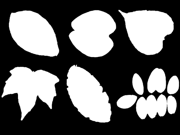


 pair as key, and the cluster as value. If the key was not found in the dictionary, we then proceeded to predict the probabilities for each cluster, added the key and cluster to the dictionary, and returned the associated cluster with the biggest probability.
 ![key ← hash(pixel[S],pixel[V ])](/img/revistas/cleiej/v19n1/1a0712x.png)

![pixelDictionary[key]](/img/revistas/cleiej/v19n1/1a0714x.png)
![probabilities← EM.predict(pixel[S],pixel[V])](/img/revistas/cleiej/v19n1/1a0715x.png)
![pixelDict[key]= probabilities[0]> probabilities[<a href=](/img/revistas/cleiej/v19n1/1a0716x.png) 1] " class="math" >
1] " class="math" > ![pixelDict[key]](/img/revistas/cleiej/v19n1/1a0717x.png)
 and
and  components, followed by a cut of the leaf image matrix to those resulting minimum and maximum coordinates. The
  was used to allow posterior algorithms ignore false positives regions that intersect the border. The results of the Clipping phase can be seen in Figure


![clipped← image[xmin :xmax,ymin:ymax]](/img/revistas/cleiej/v19n1/1a0725x.png)
 pixels. This number was used empirically based on LeafSnap’s original dataset resolution and the internal regions associated with leaf pixels. This approach means that the absolute measures of leafs are lost.


![components[0]](/img/revistas/cleiej/v19n1/1a0740x.png)


![bestCandidate← candidates[max(candidatesRatios).index]](/img/revistas/cleiej/v19n1/1a0763x.png)

 , and the leaf pixels have values of
  . First, the different contour pixels were found, then 25 different masks with disk shapes were applied on top of each contour point, providing both an area of the intersection and an arc length. Then all calculations at each scale were turned into a histogram, resulting in 25 different histograms per image, one per scale. Finally, the 25 resulting histograms were concatenated, conforming the HCoS.
  that represent the coordinates where a contour pixel was found. A contour pixel can be defined as a pixel which is surrounded by at least another pixel with the opposite color of it. Figure
 ’s and
  ’s. They were applied as masks over specific parts of the segmented leaf image (mostly contour points). The idea was to count how many pixels intersected the segmented image and each disk mask. We created two different types of disks. The first type is filled up with
  ’s, as shown in Figure
  ’s are present only in the circumference of the disk (see Figure
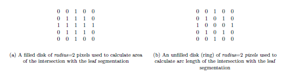


 in this case), at a given contour pixel. The gray area shows the intersection of pixels with the leaf segmentation. This procedure was then repeated over all the pixels from the contour vector in the same way.
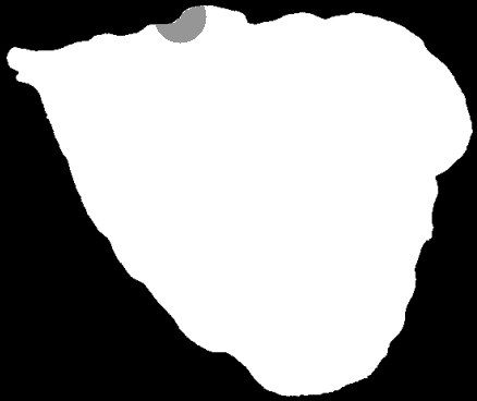

 (R2P16) implementation, and the one below shows a
  (R1P8) pixel implementation. The different variants of the LBPV used are shown in Table
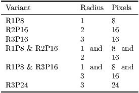
 (R2P16) and the lower one to a
  (R1P8) pattern
 corresponds the count of pixels in the leaf texture that had code
  . Also, given that the implementation is a LBPV, non-uniform codes are not used. Thus, the bin number
  is the
  feature, not just the binary code
 species, not the first
  images, as shown by Algorithm
  species


 in order to measure how different algorithms behaved as the value of
  increased.
  is the histogram intersection between a histograms
  and
and  of same size,
  is the number of bins, and
  and
and  are each a bin in histograms
  and
and  , respectively. This distance metric is also normalized to unit length.
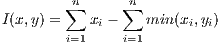
 be an identification experiment that consists of a model
  , a set
  that contains
  images of leaves of
  (not necessarily different) unknown tree species to be identified, and an integer value
  ,
,  . We define
  as a boolean function that indicates if model
  generates a ranking in which one of the top
  candidate species is a correct identification of sample
  . Equation
  .
. 
 elements is considered a test image and the remaining
  images the training subset. We used both approaches as explained at the end of this section.
  in total. However we varied the factor associated with each model to see the behavior across different combinations. We used factors of (0.10, 0.90), (0.20, 0.80), (0.30, 0.70), (0.40, 0.60), (0.50, 0.50), (0.60, 0.40), (0.70, 0.30), (0.80, 0.20), (0.90, 0.10). For example,
  means we gave the same level of importance to each model on that combination. Algorithm


![distance1 ← resultsAlgorithm1[species]](/img/revistas/cleiej/v19n1/1a07143x.png)
![distance2 ← resultsAlgorithm2[species]](/img/revistas/cleiej/v19n1/1a07144x.png)
![results[species]← (distance1*factor)+(distance2*(1- factor))](/img/revistas/cleiej/v19n1/1a07145x.png)
![combinedRanking[factor]← TakeBestKDistances(results)](/img/revistas/cleiej/v19n1/1a07146x.png)
 described in Table
  , and the following data sets: Costa Rica clean subset (One versus All,
  ), Costa Rica noisy subset (One versus All,
  ), and Costa Rica complete data set (training set with all
  clean images and testing set with all
  noisy images). In each experiment,
  was calculated for the corresponding dataset
  . In addition, for model HCoS & R1P8 & R3P16, Algorithm
  GHz, and
  GBs on RAM.
 that provides results statistically equivalent to those obtained when
  for each species? Obviously, accuracy increases as the value of
  increases. However, for practical reasons, we would like to test if there is a threshold value
  after which accuracy remains statistically equivalent to using
  . For example, in a mobile app users would appreciate if the number of best ranked species is not the maximum value 10, but a smaller number.
  HCoS and
  R1P8 & R3P16,
  HCoS and
  R1P8 & R3P16,
  HCoS and
  R1P8 & R3P16 and HCoS (curvature alone). This also includes creating clusters of species based on their most significant algorithms, and understanding the clusters with more species and best accuracies.
  . We used a confidence level of
  . Once each GLM was calculated and each main effect significance known and proven, we calculated if all levels within each factor were statistically equivalent. We are actually trying to find the levels that are significantly different, for all three factors.. We used a Tukey statistical test for each factor. Table
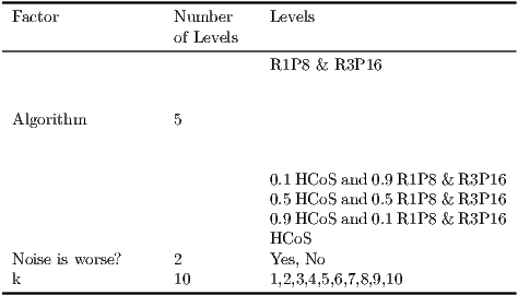

 has become an informal benchmarking value in other research
  . For this experiment, we ran a Binary Logistic Regression and optimized it, thus maximizing the probability of a successful identification. Based on the resulting regression model, we calculated the two best algorithms for both noisy and clean factors, and
  , per species.
  for a 0.991. We also attempted to use texture only, which shows to be very extremely accurate with up to 0.98. This dataset has been, however, artificially cleaned, so other studies should be evaluated on more complex datasets.
 and the model is
  HCoS and
  R1P8 & R3P16. The resulting accuracy is
  , in contrast with the accuracy of HCoS which is
  . Notice however that
  HCoS and
  R1P8 & R3P16 is also the best for all values of
  . For
. For  ,
,  HCoS and
  R1P8 & R3P16 and
  HCoS and
  R1P8 & R3P16 have very similar levels of accuracy. Figure 11 more clearly depicts these comparisons.
  HCoS and
  R1P8 & R3P16 has the best accuracy for all values of
  . In addition, the level of accuracy improvement with respect to HCoS is considerably larger, ranging from
  when
when  to
to  when
when  as shown in Table
 ![[14.5%,43.9% ]](/img/revistas/cleiej/v19n1/1a07198x.png) range.
range. 
 . Overall, the best combination seems to be
  HCoS and
  LBPV. It is also important to notice how the accuracy is sensitive to the quality of the dataset. The clean subset has a tendency to improve the recognition accuracy, in contrast with the noisy subset. This reflects the importance of good pre-processing and good segmentation. Shadows, dust, and other artifacts affect the final accuracy results.
  is that the accuracy of the implementation of HCoS equals the ones obtained by combining curvature and texture. In contrast, our alternative hypothesis
  is that the accuracy of the implementation of HCoS is less than the combinations.
  resulted in very low p-Values, which reject
  . However a few accuracy increases from
  HCoS and
  R1P8 & R3P16 did fail the test. This means that, as the weight increases for HCoS, it starts getting non-significant accuracy increases, which makes sense since it is almost equal to HCoS alone.
  .
.  . For
. For  the results are not significant. ]]>


 to
to  seconds. However, the median of the elapsed time is
  seconds for the clean subset and
  seconds for the noisy subset. These are suitable times even for mobile applications that use the developed back-end.
 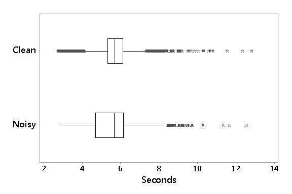 ]]>
]]>

 ” indicates the threshold value
  per species. As indicated before, any
  will be slightly better, but this is not statistically significant.


 is achieved by species
  .
.  .
.  . Overall, 13 species show a
  value, while 20 species have
  , and the rest result in
  . As
. As  is lower, then the potential maximum accuracy for that species tends to be very high.
  HCoS and
  R1P8 & R3P16. Some also have R1P8 & R3P16 which is texture alone without curvature.
  HCoS and
  R1P8 & R3P16, and have the second best accuracy across all species. The very best cluster is Cluster 9, reaching an Accuracy of
  .
. 
 HCoS and
  R1P8 & R3P16 combination, and
  HCoS and
  R1P8 & R3P16 combination. This means both of them are statistically equivalent for these species.
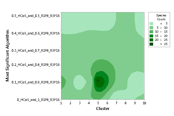


 and the noisy dataset is used. Most algorithms are combinations, from pure texture, to a
  HCoS and
  R1P8 & R3P16 combination. No combination gets near a pure curvature algorithm. Similar results are noted in Figure
  HCoS and
  R1P8 & R3P16 combination. In general the distribution is very homogenous.
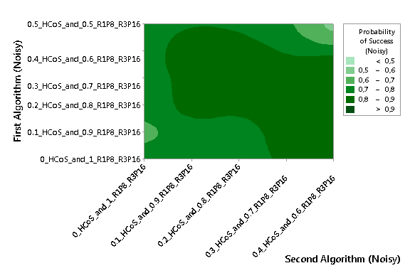


 and the clean dataset is used. In this case the best algorithms per species are more spread across most combinations. This is due the lack of noise in the data and the lesser affectation of the curvature algorithms. This, compared with the data of Table
  HCoS and
  R1P8 & R3P16 combination.
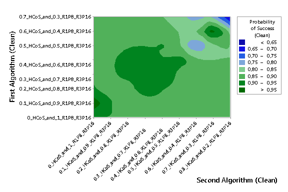


 HCoS and
  R1P8 & R3P16, for the Costa Rican clean subset, the improvement ranges from
  to
to  , depending on the value of
  . Similarly, with the noisy subset, the improvement ranges from
  to
to  . These improvements were proved to be statistically significant in our experiments.
  , i.e., the size of the set of candidates that are considered best possibilities in an identification process, good levels of accuracy were obtained for
  in 63% of the species. Working with noisy images had a negative effect on levels of accuracy on 61 out of 65 species studied, as compared to clean images and a clean dataset. Finally, texture also stands out in most individual cases as the determining factor for high accuracy levels as compared to leaf shape.
  did not render a clear winner but highlighted that the best combination of algorithms should use weigths smaller than 0.2 to HCoS.