<?xml version="1.0" encoding="ISO-8859-1"?><article xmlns:mml="http://www.w3.org/1998/Math/MathML" xmlns:xlink="http://www.w3.org/1999/xlink" xmlns:xsi="http://www.w3.org/2001/XMLSchema-instance">
<front>
<journal-meta>
<journal-id>0717-5000</journal-id>
<journal-title><![CDATA[CLEI Electronic Journal]]></journal-title>
<abbrev-journal-title><![CDATA[CLEIej]]></abbrev-journal-title>
<issn>0717-5000</issn>
<publisher>
<publisher-name><![CDATA[Centro Latinoamericano de Estudios en Informática]]></publisher-name>
</publisher>
</journal-meta>
<article-meta>
<article-id>S0717-50002013000200003</article-id>
<title-group>
<article-title xml:lang="en"><![CDATA[Virtual Colonoscopy]]></article-title>
</title-group>
<contrib-group>
<contrib contrib-type="author">
<name>
<surname><![CDATA[Poó]]></surname>
<given-names><![CDATA[María]]></given-names>
</name>
<xref ref-type="aff" rid="A01"/>
</contrib>
<contrib contrib-type="author">
<name>
<surname><![CDATA[Buysee]]></surname>
<given-names><![CDATA[Eduardo]]></given-names>
</name>
<xref ref-type="aff" rid="A01"/>
</contrib>
<contrib contrib-type="author">
<name>
<surname><![CDATA[Carmona]]></surname>
<given-names><![CDATA[Rhadamés]]></given-names>
</name>
<xref ref-type="aff" rid="A01"/>
</contrib>
<contrib contrib-type="author">
<name>
<surname><![CDATA[Coto]]></surname>
<given-names><![CDATA[Ernesto]]></given-names>
</name>
<xref ref-type="aff" rid="A01"/>
</contrib>
<contrib contrib-type="author">
<name>
<surname><![CDATA[Navarro]]></surname>
<given-names><![CDATA[Héctor]]></given-names>
</name>
<xref ref-type="aff" rid="A01"/>
</contrib>
</contrib-group>
<aff id="A01">
<institution><![CDATA[,Universidad Central de Venezuela Centro de Computación Gráfica Escuela de Computación]]></institution>
<addr-line><![CDATA[ ]]></addr-line>
<country>Venezuela</country>
</aff>
<pub-date pub-type="pub">
<day>00</day>
<month>08</month>
<year>2013</year>
</pub-date>
<pub-date pub-type="epub">
<day>00</day>
<month>08</month>
<year>2013</year>
</pub-date>
<volume>16</volume>
<numero>2</numero>
<fpage>3</fpage>
<lpage>3</lpage>
<copyright-statement/>
<copyright-year/>
<self-uri xlink:href="http://www.scielo.edu.uy/scielo.php?script=sci_arttext&amp;pid=S0717-50002013000200003&amp;lng=en&amp;nrm=iso"></self-uri><self-uri xlink:href="http://www.scielo.edu.uy/scielo.php?script=sci_abstract&amp;pid=S0717-50002013000200003&amp;lng=en&amp;nrm=iso"></self-uri><self-uri xlink:href="http://www.scielo.edu.uy/scielo.php?script=sci_pdf&amp;pid=S0717-50002013000200003&amp;lng=en&amp;nrm=iso"></self-uri><abstract abstract-type="short" xml:lang="en"><p><![CDATA[Nowadays, Virtual Colonoscopy (VC) is an important non-invasive alternative for the study of the colon. Substantial research efforts have been dedicated to this method, and one of the major challenges has always been producing accurate results in a short period of time. One of the most crucial phases of VC is the detection of polyp candidates, where possible lesions on the colon walls are automatically detected. Frequently, this stage requires intensive computations and therefore it is important to develop new techniques for reducing its execution time. This paper presents a technique for automatic detection of polyp candidates based on curvature analysis that reduces the execution time using parallel programming in CUDA. Additionally, we introduce a novel technique for discarding false positive detections based on the shape of a candidate in a planar cut. The obtained results show a remarkable reduction in execution time with respect to a CPU implementation as well as a low rate of false positives.]]></p></abstract>
<abstract abstract-type="short" xml:lang="es"><p><![CDATA[Actualmente, la Colonoscopia Virtual (CV) es una importante alternativa no-invasiva para el estudio del colon. A este método se le han dedicado sustanciales esfuerzos de investigación, y uno de los mayores restos siempre ha sido el de producir resultados precisos en un periodo corto de tiempo. Una de las fases más cruciales de la CV es la detección de candidatos a pólipos, donde se detectan automáticamente posibles lesiones en las paredes del colon. Frecuentemente, esta etapa requiere cálculos intensivos y por lo tanto es importante desarrollar nuevas técnicas para reducir su tiempo de ejecución. Este trabajo presenta una técnica para la detección automática de candidatos a pólipo basada en análisis de curvatura que reduce su tiempo de ejecución usando programación paralela en CUDA. Adicionalmente, se introduce una técnica novedosa para descartar falsos positivos basada en la forma de un candidato en un corte planar. Los resultados obtenidos muestran una reducción notable del tiempo de ejecución con respecto a una implementación para CPU, así como también una baja tasa de falsos positivos.]]></p></abstract>
<kwd-group>
<kwd lng="en"><![CDATA[Virtual Colonoscopy]]></kwd>
<kwd lng="en"><![CDATA[Polyp Detection]]></kwd>
<kwd lng="en"><![CDATA[Curvature Analysis]]></kwd>
<kwd lng="en"><![CDATA[CUDA]]></kwd>
<kwd lng="es"><![CDATA[Colonoscopia Virtual]]></kwd>
<kwd lng="es"><![CDATA[Detección de Pólipos]]></kwd>
<kwd lng="es"><![CDATA[Análisis de Curvatura]]></kwd>
<kwd lng="es"><![CDATA[CUDA]]></kwd>
</kwd-group>
</article-meta>
</front><body><![CDATA[ <div class=Section1>      <p style='margin:0cm;margin-bottom:.0001pt;mso-pagination:widow-orphan'><b> <font face="Verdana" size="4"><a name="_GoBack"></a></font><span lang=EN-US style='mso-bidi-font-size: 10.0pt'><font face="Verdana" size="4">GPU-accelerated Polyp Detection in Virtual Colonoscopy</font></span></b><o:p></o:p></p>  </div>  <b style='mso-bidi-font-weight:normal'> <span lang=EN-US style='font-size:10pt; mso-bidi-font-size:10.0pt;font-family:"Verdana";mso-fareast-font-family: "Times New Roman";mso-ansi-language:EN-US;mso-fareast-language:AR-SA; mso-bidi-language:AR-SA'><br clear=all style='page-break-before:auto; mso-break-type:section-break'> </span></b>      <div class=Section2>      <p align=center style='text-align:center;mso-pagination:widow-orphan; tab-stops:center 85.0pt 261.0pt 414.0pt'><span lang=EN-US style='font-size: 10.0pt;font-style:normal'><font face="Verdana"><![if !supportEmptyParas]>&nbsp;<![endif]></font><o:p></o:p></span></p>      <p align=center style='text-align:center;mso-pagination:widow-orphan; tab-stops:center 85.0pt 261.0pt 414.0pt'><b style='mso-bidi-font-weight:normal'><span lang=EN-US style='font-size:10.0pt;font-style:normal'><font face="Verdana"><![if !supportEmptyParas]>&nbsp;<![endif]></font><o:p></o:p></span></b></p>      <p align=center style='text-align:center;mso-pagination:widow-orphan; tab-stops:center 85.0pt 261.0pt 414.0pt'><b style='mso-bidi-font-weight:normal'><span lang=ES-VE style='mso-ansi-language:ES-VE;font-style:normal'> <font face="Verdana" size="2">María Poó, Eduardo Buysee, Rhadamés Carmona, </font> <o:p></o:p></span></b></p>      <p align=center style='text-align:center;mso-pagination:widow-orphan; tab-stops:center 85.0pt 261.0pt 414.0pt'><font face="Verdana"><b style='mso-bidi-font-weight:normal'><span lang=ES-VE style='mso-ansi-language:ES-VE;font-style:normal'><font size="2">Ernesto Coto </font> </span></b></font><span lang=ES-VE style='mso-ansi-language:ES-VE;font-style:normal'> <font face="Verdana" size="2">and</font><b style='mso-bidi-font-weight:normal'><font size="2" face="Verdana"> Héctor Navarro </font> <o:p></o:p></b></span></p>      <p align=center style='text-align:center;mso-pagination:widow-orphan; tab-stops:center 85.0pt 261.0pt 414.0pt'><span lang=ES-VE style='mso-ansi-language: ES-VE;font-style:normal'><font face="Verdana" size="2">Centro de Computación Gráfica, Universidad Central de Venezuela</font><o:p></o:p></span></p>      <p align=center style='text-align:center;mso-pagination:widow-orphan; tab-stops:center 85.0pt 261.0pt 414.0pt'><span lang=ES-VE style='mso-ansi-language: ES-VE;font-style:normal'><font face="Verdana" size="2">Escuela de Computación, Caracas, Venezuela, 1041-A</font><o:p></o:p></span></p>      <p align=center style='text-align:center;mso-pagination:widow-orphan; tab-stops:center 85.0pt 261.0pt 414.0pt'><span lang=ES-VE style='mso-bidi-font-size: 12.0pt;mso-ansi-language:ES-VE'><font face="Verdana" size="2"><a href="malenapoo@hotmail.com">malenapoo@hotmail.com</a>, <a href="elchuck81@gmail.com">elchuck81@gmail.com</a>,</font><o:p></o:p></span></p>      ]]></body>
<body><![CDATA[<p align=center style='text-align:center;mso-pagination:widow-orphan; tab-stops:center 85.0pt 261.0pt 414.0pt'><font face="Verdana"><span lang=ES-VE style='mso-bidi-font-size: 12.0pt;mso-ansi-language:ES-VE;font-style:normal'><font size="2">{</font></span><font size="2"><span lang=ES-VE style='mso-bidi-font-size:12.0pt;mso-ansi-language:ES-VE'><a href="mailto:rhadames.carmona@ciens.ucv.ve">rhadames.carmona</a>, <a href="mailto:ernesto.coto@ciens.ucv.ve">ernesto.coto</a>, <a href="mailto:hector.navarro@ciens.ucv.ve">hector.navarro</a></span><span lang=ES-VE style='mso-bidi-font-size:12.0pt;mso-ansi-language:ES-VE;font-style: normal'>}</span></font></font><span lang=ES-VE style='mso-bidi-font-size:12.0pt;mso-ansi-language: ES-VE'><font face="Verdana"><font size="2">@ciens.ucv.ve</font></font><o:p></o:p></span></p>  </div>  <i style='mso-bidi-font-style:normal'> <span style='font-size:10pt;mso-bidi-font-size: 10.0pt;font-family:"Verdana";mso-fareast-font-family:"Times New Roman"; mso-ansi-language:ES;mso-fareast-language:AR-SA;mso-bidi-language:AR-SA'><br clear=all style='page-break-before:auto;mso-break-type:section-break'> </span></i>      <div class=Section3></div>  <span style='font-size:10.0pt;font-family:"Verdana";mso-fareast-font-family: "Times New Roman";mso-ansi-language:ES;mso-fareast-language:AR-SA;mso-bidi-language: AR-SA'><br clear=all style='page-break-before:auto;mso-break-type:section-break'> </span>      <div class=Section4>      <p style='margin-top:12.0pt;margin-right:45.35pt;margin-bottom: 6.0pt;margin-left:45.35pt'><font face="Verdana" size="2"><span lang=EN-US>Abstract</span></font></p>      <p style='margin-top:0cm;margin-right:45.0pt;margin-bottom: 0cm;margin-left:45.0pt;margin-bottom:.0001pt;text-align:justify'><span lang=EN-US style='font-size:10.0pt;mso-bidi-font-size:12.0pt;mso-ansi-language: EN-US'><font face="Verdana">Nowadays, Virtual Colonoscopy (VC) is an important non-invasive alternative for the study of the colon. Substantial research efforts have been dedicated to this method, and one of the major challenges has always been producing accurate results in a short period of time. One of the most crucial phases of VC is the detection of polyp candidates, where possible lesions on the colon walls are automatically detected. Frequently, this stage requires intensive computations and therefore it is important to develop new techniques for reducing its execution time. This paper presents a technique for automatic detection of polyp candidates based on curvature analysis that reduces the execution time using parallel programming in CUDA. Additionally, we introduce a novel technique for discarding false positive detections based on the shape of a candidate in a planar cut. The obtained results show a remarkable reduction in execution time with respect to a CPU implementation as well as a low rate of false positives. </font> <o:p></o:p></span></p>  </div>  <span style='font-size:10.0pt;font-family:"Verdana";mso-fareast-font-family: "Times New Roman";mso-ansi-language:ES;mso-fareast-language:AR-SA;mso-bidi-language: AR-SA'><br clear=all style='page-break-before:auto;mso-break-type:section-break'> </span>      <div class=Section5>      <p style='margin-top:12.0pt;margin-right:45.35pt;margin-bottom: 6.0pt;margin-left:45.35pt'><span style='mso-ansi-language:ES'> <font face="Verdana" size="2">Spanish abstract</font><o:p></o:p></span></p>      <p style='margin-top:0cm;margin-right:45.0pt;margin-bottom: 0cm;margin-left:45.0pt;margin-bottom:.0001pt;text-align:justify'><span style='font-size:10.0pt;mso-bidi-font-size:12.0pt'><font face="Verdana">Actualmente, la Colonoscopia Virtual (CV) es una importante alternativa no-invasiva para el estudio del colon. A este método se le han dedicado sustanciales esfuerzos de investigación, y uno de los mayores restos siempre ha sido el de producir resultados precisos en un periodo corto de tiempo. Una de las fases más cruciales de la CV es la detección de candidatos a pólipos, donde se detectan automáticamente posibles lesiones en las paredes del colon. Frecuentemente, esta etapa requiere cálculos intensivos y por lo tanto es importante desarrollar nuevas técnicas para reducir su tiempo de ejecución. Este trabajo presenta una técnica para la detección automática de candidatos a pólipo basada en análisis de curvatura que reduce su tiempo de ejecución usando programación paralela en CUDA. Adicionalmente, se introduce una técnica novedosa para descartar falsos positivos basada en la forma de un candidato en un corte planar. Los resultados obtenidos muestran una reducción notable del tiempo de ejecución con respecto a una implementación para CPU, así como también una baja tasa de falsos positivos.</font><o:p></o:p></span></p>      <p style='margin-top:0cm;margin-right:45.0pt;margin-bottom: 0cm;margin-left:45.0pt;margin-bottom:.0001pt;text-align:justify'><span style='font-size:10.0pt;mso-bidi-font-size:12.0pt'><font face="Verdana"><![if !supportEmptyParas]>&nbsp;<![endif]></font><o:p></o:p></span></p>      <p style='margin-right:45.0pt;text-align:justify;mso-list:none;tab-stops:35.4pt'> <span lang=EN-US style='font-size:10.0pt;mso-bidi-font-size:12.0pt;font-family:"Verdana"; mso-ansi-language:EN-US'>Keywords: </span><font face="Verdana"> <span lang=EN-US style='font-size: 10.0pt;mso-bidi-font-size:12.0pt;mso-ansi-language: EN-US;font-weight:normal'>Virtual Colonoscopy, Polyp Detection, Curvature Analysis, CUDA. </span></font> <o:p></o:p></p>      ]]></body>
<body><![CDATA[<p><span lang=EN-US style='mso-ansi-language:EN-US'> <font face="Verdana" size="2"><![if !supportEmptyParas]>&nbsp;<![endif]></font><o:p></o:p></span></p>      <p style='margin-right:45.0pt;text-align:justify;mso-list:none;tab-stops:35.4pt'> <span style='font-size:10.0pt;mso-bidi-font-size:12.0pt;font-family:"Verdana"'>Spanish Keywords: </span> <span style='font-size:10.0pt;mso-bidi-font-size:12.0pt; font-weight:normal'><font face="Verdana">Colonoscopia Virtual, Detección de Pólipos, Análisis de Curvatura, CUDA</font></span><o:p></o:p></p>      <p style='margin-top:0cm;margin-right:45.0pt;margin-bottom:0cm;margin-left: 45.0pt;margin-bottom:.0001pt;text-align:justify'><![if !supportLists]> <span style='font-style:normal; font-variant:normal; font-weight:normal; font-size:10pt; font-family:Verdana; mso-bidi-font-size:12.0pt'>&nbsp;&nbsp;&nbsp;&nbsp;&nbsp;&nbsp;&nbsp; </span><![endif]> <span style='font-size:10.0pt;mso-bidi-font-size:12.0pt; font-weight:normal'><![if !supportEmptyParas]><font face="Verdana">&nbsp;</font><![endif]></span><o:p></o:p></p>      <p style='margin-right:45.0pt;text-align:justify;mso-list:none;tab-stops:35.4pt'> <font face="Verdana"> <span lang=EN-US style='font-size:10.0pt;mso-bidi-font-size:12.0pt;mso-ansi-language:EN-US;font-weight:normal'>Received 2012-05-30, Revised 2013-01-15</span></font><o:p></o:p></p>      <p style='text-align:justify'><span lang=EN-US style='font-size:10.0pt;mso-bidi-font-size:12.0pt;mso-ansi-language:EN-US'> <font face="Verdana"><![if !supportEmptyParas]>&nbsp;<![endif]></font><o:p></o:p></span></p>      <p style='margin-top:0cm;margin-right:0cm;margin-bottom:5.95pt;margin-left: 0cm;text-align:justify;text-indent:0cm;mso-list:none;tab-stops:35.4pt'><b style='mso-bidi-font-weight:normal'><font face="Verdana"> <span lang=EN-US style='font-size:10pt; font-variant:normal;mso-ansi-language:EN-US'>1 Introduction</span></font><o:p></o:p></b></p>      <p style='text-align:justify;mso-hyphenate:auto;mso-layout-grid-align: none;text-autospace:none'><font face="Verdana"><span lang=EN-US style='font-size:10.0pt;mso-ansi-language: EN-US'>Cancer is the generic name for a group of diseases consisting on the division and abnormal reproduction of body cells. <span style='mso-bidi-font-style: italic'>Cancers are named after the part of the body</span> where they start. When the cancer starts at the </span><span lang=EN-US style='font-size:10.0pt; mso-ansi-language:EN-US;mso-fareast-language:ES-VE'>colon or rectum is called <i style='mso-bidi-font-style:normal'>colon cancer</i> or<i> colorectal cancer</i>. </span></font><span lang=EN-US style='font-size:10.0pt;mso-ansi-language:EN-US'> <font face="Verdana">Nowadays, hundreds of persons in Venezuela <a href="#r1">(1)</a> and millions worldwide <a href="#r2">(2)</a> die of colon cancer. This type of cancer is related to the abnormal growth of tissue at the mucous that covers the colon wall, called a <i style='mso-bidi-font-style:normal'>colorectal polyp</i>. The most common type of polyp is a <i style='mso-bidi-font-style: normal'>metaplastic polyp</i>, in which cells change from one normal type to another. They have almost no risk of becoming malignant. <i style='mso-bidi-font-style: normal'>Adenomatous polyps</i> can become malignant. If these polyps are not detected and extracted on an early stage they can degenerate and transform into cancer.</font><o:p></o:p></span></p>      <p style='text-align:justify;text-indent:18.15pt;mso-hyphenate: auto;mso-layout-grid-align:none;text-autospace:none'><span lang=EN-US style='font-size:10.0pt;mso-ansi-language:EN-US'><font face="Verdana">An optical colonoscopy is the gold standard examination for searching polyps in a patient’s colon. However, this procedure is very invasive and uncomfortable for the patient. <i style='mso-bidi-font-style:normal'>Virtual</i> <i style='mso-bidi-font-style: normal'>Colonoscopy</i> is an excellent non-invasive alternative for colon polyp detection. In Virtual Colonoscopy, images from the patient’s colon are captured with a <i style='mso-bidi-font-style:normal'>Computer</i> <i style='mso-bidi-font-style:normal'>Tomography</i> (CT) <i style='mso-bidi-font-style: normal'>Colonography</i> and these images are then processed and virtually browsed in a computer, searching for polyp candidates.</font><o:p></o:p></span></p>      <p style='text-align:justify;text-indent:18.15pt;mso-hyphenate: auto;mso-layout-grid-align:none;text-autospace:none'><font face="Verdana"><span lang=EN-US style='font-size:10.0pt;mso-ansi-language:EN-US'>Typically, </span><span lang=EN-US style='font-size:10.0pt;mso-ansi-language:EN-US;mso-fareast-language: ES-VE'>VC m</span><span lang=EN-US style='font-size:10.0pt;mso-ansi-language: EN-US'>edical </span><span lang=EN-US style='font-size:10.0pt;mso-ansi-language: EN-US;mso-fareast-language:ES-VE'>workstations</span><span lang=EN-US style='font-size:10.0pt;mso-ansi-language:EN-US'> provide an automatic virtual </span><span lang=EN-US style='font-size:10.0pt;mso-ansi-language:EN-US;mso-fareast-language: ES-VE'>flythrough inside the colon, which the doctor can stop at any moment and move the virtual colonoscope freely inside the colon. This searching procedure has been proved effective but it is well known that it can consume a considerable amount of time to examine the complete extent of the colon. Therefore, automatic polyp detection has been suggested as a method for rapidly pointing out relevant areas of the colon to the medical doctor.</span></font><span lang=EN-US style='font-size:10.0pt;mso-ansi-language:EN-US'><font face="Verdana"> Several polyp detection methods have been proposed in the literature. Among others we can mention methods based on curvature analysis <a href="#r3">(3)</a><a href="#r4">(4)</a><a href="#r5">(5)</a>, curvature lines <a href="#r6">(6)</a><a href="#r4">(4)</a>, surface adjustment <a href="#r7">(7)</a>, heat diffusion fields <a href="#r8">(8)</a> and water-planes <a href="#r9">(9)</a>. All these techniques require a lot of computations, producing long response times.</font><o:p></o:p></span></p>      <p style='text-align:justify;text-indent:18.0pt;mso-pagination: none'><span lang=EN-US style='font-size:10.0pt;mso-ansi-language:EN-US'> <font face="Verdana">In this work, we present the parallelization of the algorithm for automatic polyp detection method based on curvature analysis proposed by Yoshida and Nappi <a href="#r3">(3)</a>. In this method, a shape index is computed for each voxel on the colon wall, which requires the approximation of first and second order partial derivatives, where intensive computations are needed. These derivatives are implemented in a parallel algorithm using CUDA <a href="#r10">(10)</a>, taking advantage of current NVidia’s <i style='mso-bidi-font-style:normal'>Graphics</i> <i style='mso-bidi-font-style: normal'>Processing</i> <i style='mso-bidi-font-style:normal'>Units</i> (GPUs). Since curvature analysis can generate numerous false positives, in this work we also propose a strategy for discarding false positives by studying the shape of the polyp candidate in a longitudinal cut. Several tests were performed on CT Colonography scans showing an excellent response time reduction, as well as an effective decrease of false positives.</font><o:p></o:p></span></p>      ]]></body>
<body><![CDATA[<p style='text-align:justify;text-indent:18.15pt'><font face="Verdana"><span lang=EN-US style='font-size:10.0pt;mso-ansi-language:EN-US'>The following section describes previous works on automatic polyp detection and the parallelization of VC algorithms with CUDA, and then we describe our new variation of </span><span lang=EN-US style='font-size:10.0pt;mso-bidi-font-size: 12.0pt;mso-ansi-language:EN-US'>Yoshida and Nappi’s </span></font><span lang=EN-US style='font-size:10.0pt;mso-ansi-language:EN-US'><font face="Verdana">method <a href="#r3">(3)</a> and its CUDA implementation on Section 3. Following this, we describe tests and results of our method over six CT Colonography datasets in Section 4. Finally, conclusions and future work are described in Section 5.</font><o:p></o:p></span></p>      <p style='text-align:justify;text-indent:18.15pt'><b style='mso-bidi-font-weight:normal'><span lang=EN-US style='font-size:10.0pt; mso-bidi-font-size:12.0pt;mso-ansi-language:EN-US'><font face="Verdana"><![if !supportEmptyParas]>&nbsp;<![endif]></font><o:p></o:p></span></b></p>      <p style='margin-top:0cm;margin-right:0cm;margin-bottom:5.95pt;margin-left: 0cm;text-align:justify;text-indent:0cm;mso-pagination:none;page-break-after: auto;mso-list:none;tab-stops:35.4pt'><b><font face="Verdana"> <span lang=EN-US style='font-size:10pt; font-variant:normal;mso-ansi-language:EN-US'>2 Previous Works</span></font><o:p></o:p></b></p>      <p style='margin:0cm;margin-bottom:.0001pt;text-align:justify;mso-pagination: none'><font face="Verdana"><span lang=EN-US style='font-size:10.0pt'>There are several methods for polyp detection on volumetric data. These methods usually implement two phases. The first phase detects polyp candidates, where structures that might be polyps are detected. On the second phase false positives are discarded.</span></font><span lang=EN-US style='font-size:10.0pt;mso-bidi-font-size:12.0pt'><o:p></o:p></span></p>      <p style='text-align:justify;text-indent:18.15pt'><span lang=EN-US style='font-size:10.0pt;mso-bidi-font-size:12.0pt;mso-ansi-language: EN-US'><font face="Verdana">In order to detect polyp candidates, Yoshida and Nappi <a href="#r3">(3)</a> proposed in 2001 a method based on curvatures that extracts a thick region of the colon wall to eliminate the largest possible amount of false positives. This method extracts 3D geometric attributes of the polyps using a shape index and a curvature index, grouping polyp candidates and then determining other attributes that might help reducing false positives. That same year, Gokturk and Tomasi <a href="#r11">(11)</a> used a <i style='mso-bidi-font-style:normal'>Support Vector Machine</i> (SVM) to eliminate false positives. They used orthogonal planes in the polyp candidate, and extract geometric features that feed the SVM in the training. They also consider voxel intensity to feed up the classifier. </font> <o:p></o:p></span></p>      <p style='text-align:justify;text-indent:18.15pt'><span lang=EN-US style='font-size:10.0pt;mso-bidi-font-size:12.0pt;mso-ansi-language: EN-US'><font face="Verdana">In 2004, Paik et al. <a href="#r12">(12)</a> introduced an algorithm called <i style='mso-bidi-font-style:normal'>Surface Normal Overlap</i> (SNO), which is used for colonic polyp detection as well as for lung nodule detection in CT images. Their approach computes for each voxel a score proportional to the number of surface normals that pass through or near it. They noticed that polyp voxels tend to have a higher score than other voxels, due to the presence of convex regions in the surface of polyps.</font><o:p></o:p></span></p>      <p style='text-align:justify;text-indent:18.15pt'><span lang=EN-US style='font-size:10.0pt;mso-bidi-font-size:12.0pt;mso-ansi-language: EN-US'><font face="Verdana">In 2005, Kitasaka et al. <a href="#r7">(7)</a> proposed a polyp detection method computing the curvature by means of surface fitting. At each voxel of the colon wall, a second degree polynomial <i style='mso-bidi-font-style:normal'>f</i>(<i style='mso-bidi-font-style:normal'>x</i>,<i style='mso-bidi-font-style:normal'>y</i>,<i style='mso-bidi-font-style:normal'>z</i>) is fitted to the voxel’s neighborhood, using minimum squares. Changing the size of the neighborhood allows the detection of polyps with different sizes. The authors report they found less false positives than applying the curvature based method. That same year, Bitter et al. <a href="#r9">(9)</a> proposed the <i style='mso-bidi-font-style:normal'>water-plane</i> method. This method works over a triangulated surface mesh of the colon, extracted from the CT data. The method simulates that the colon wall is being filled up with water from a vertex on the mesh, from the outside of the colon, until the water starts to spill out. The idea is finding the set of vertexes that form an almost convex volume. According to their tests, good candidates contain at least 20 vertexes.</font><o:p></o:p></span></p>      <p style='text-align:justify;text-indent:18.15pt;mso-pagination: none'><span lang=EN-US style='font-size:10.0pt;mso-bidi-font-size:12.0pt; mso-ansi-language:EN-US'><font face="Verdana">In 2006 Zhao et al. <a href="#r6">(6)</a> introduced a technique for characterizing and visualizing curvature lines on the colon surface in order to detect polyps. The basic idea is to show the colon surface using a local illumination model, and enhance it by displaying the curvature of these surfaces. This method works on the surface mesh of a colon extracted with the <i style='mso-bidi-font-style:normal'>marching cubes</i> technique <a href="#r13">(13)</a>, and with implicit iso-surfaces. The main advantage of this technique is that it allows enhancing virtual colonoscopy images by adding the curvature lines which allows the radiologist to easily characterize polyps. However, this method has not been adapted to automatic polyp detection.</font><o:p></o:p></span></p>      <p style='text-align:justify;text-indent:18.15pt;mso-pagination: none'><span lang=EN-US style='font-size:10.0pt;mso-bidi-font-size:12.0pt; mso-ansi-language:EN-US'><font face="Verdana">Later in 2007, Konukoglu et al. <a href="#r8">(8)</a> proposed to use <i style='mso-bidi-font-style:normal'>Heat Diffusion Fields</i> (HDFs) for polyp detection. The main idea is using the heat diffusion process to generate a vector field which is correlated with the shape of the colon wall. They found that the heat diffusion process generates a diffusion pattern singularity near the centers of protruding structures, like polyps. They suppose an improvement of Yoshida's method, but a direct comparison between both methods is not included. The main drawback of this method is its high computational requirements.</font><o:p></o:p></span></p>      <p style='text-align:justify;text-indent:18.15pt;mso-pagination: none'><span lang=EN-US style='font-size:10.0pt;mso-bidi-font-size:12.0pt; mso-ansi-language:EN-US'><font face="Verdana">In 2008, Huang et al. <a href="#r5">(5)</a> researched on the use of the <i style='mso-bidi-font-style:normal'>Pareto front</i> for evaluating and enhancing region growing algorithms based on curvature, commonly used for detecting polyp candidates. They evaluated and proposed an improvement of Yoshida and Nappi’s work <a href="#r3">(3)</a> and also reported a reduction of 92% in the number of false positives in comparison with the method of Paik et al. <a href="#r12">(12)</a>.</font><o:p></o:p></span></p>      ]]></body>
<body><![CDATA[<p style='text-align:justify;text-indent:18.15pt;mso-pagination: none'><span lang=EN-US style='font-size:10.0pt;mso-bidi-font-size:12.0pt; mso-ansi-language:EN-US'><font face="Verdana">The works previously described show that it is possible to detect polyps using the explicit representation (surface or mesh), or an implicit representation (a set of grayscale values) of the colon wall. Van Ravesteijn et al. <a href="#r4">(4)</a> presented in 2009 a pattern for recognizing polyps, which combines the two types of representations and reveals that they are somehow complementary. Each of these approaches characterizes different aspects of the candidates, which are detected by means of the deformation of an explicit representation of the colon surface, or by the modification of the intensity data that contains an implicit representation. </font> <o:p></o:p></span></p>      <p style='text-align:justify;text-indent:18.15pt;mso-pagination: none'><font face="Verdana"><span lang=FR style='font-size:10.0pt;mso-bidi-font-size:12.0pt; mso-ansi-language:FR'>Qui et al. </span></font><span lang=EN-US style='font-size:10.0pt; mso-bidi-font-size:12.0pt;mso-ansi-language:EN-US'><font face="Verdana"><a href="#r14">(14)</a> implemented an algorithm of dissection and flattening of the colon (<i style='mso-bidi-font-style:normal'>Virtual Colon Flattening</i>) using CUDA. In our case, we use CUDA for accelerating the computation of the first and second derivatives, which are needed for computing the curvatures on each voxel of the colon walls. Our work is based on the parallelization of the curvature analysis, whose sequential version is presented in Yoshida and Nappi <a href="#r3">(3)</a>. The technique is complemented with a heuristic for reducing false positives.</font><o:p></o:p></span></p>      <p style='margin-top:0cm;margin-right:0cm;margin-bottom:5.95pt;margin-left: 0cm;text-align:justify;text-indent:0cm;mso-pagination:none;page-break-after: auto;mso-list:none;tab-stops:35.4pt'><b style='mso-bidi-font-weight:normal'> <font face="Verdana"> <span lang=EN-US style='font-size:10pt;font-variant: normal;mso-ansi-language:EN-US'>3 Method</span></font><o:p></o:p></b></p>      <p style='text-align:justify;mso-pagination:none'><span lang=EN-US style='font-size:10.0pt;mso-bidi-font-size:12.0pt;mso-ansi-language: EN-US'><font face="Verdana">In this work we parallelized the work of <a href="#r3">(3)</a> to determine polyp candidates. Initially, the patient’s colon is segmented using a region-growing algorithm. After this, the voxels on the surface of the colon wall are obtained. These voxels are classified according to their curvature, and grouped together to generate an initial list of polyp candidates. This list is then refined, removing false positives by studying the shape of the polyp candidate on a longitudinal cut. The elements remaining in the list correspond to the polyp candidates detected by the method. In the following, we describe in detail each of the phases of the method.</font><o:p></o:p></span></p>      <p style='text-align:justify'><span lang=EN-US style='font-size:10.0pt;mso-bidi-font-size:12.0pt;mso-ansi-language:EN-US'> <font face="Verdana"><![if !supportEmptyParas]>&nbsp;<![endif]></font><o:p></o:p></span></p>      <p style='margin-bottom:5.95pt;text-align:justify;mso-list:none;tab-stops: 35.4pt'><font face="Verdana"> <span lang=EN-US style='font-size:10.0pt;mso-bidi-font-size:12.0pt; mso-ansi-language:EN-US'>3.1 Volume Segmentation</span></font><o:p></o:p></p>      <p style='text-align:justify'><span lang=EN-US style='font-size:10.0pt;mso-bidi-font-size:12.0pt;mso-ansi-language:EN-US'> <font face="Verdana">In order to segment the volume, an intensity-based region-growing algorithm was used. The algorithm starts growing from a seed voxel inside the colon lumen with an intensity corresponding to air, and then it starts growing through the neighboring air voxels. The growing process stops when it hits the voxels of the colon wall. This process is described in more detail in <a href="#r15">(15)</a>. Once the air voxels are grouped, the resulting subvolume is dilated until the voxels of the colon walls are obtained.</font><o:p></o:p></span></p>      <p style='text-align:justify'><span lang=EN-US style='font-size:10.0pt;mso-bidi-font-size:12.0pt;mso-ansi-language:EN-US'> <font face="Verdana"><![if !supportEmptyParas]>&nbsp;<![endif]></font><o:p></o:p></span></p>      <p style='margin-top:0cm;margin-right:0cm;margin-bottom:5.95pt;margin-left: 0cm;text-align:justify;text-indent:0cm;mso-list:none;tab-stops:35.4pt'> <font face="Verdana"> <span lang=EN-US style='font-size:10.0pt;mso-bidi-font-size:12.0pt;mso-ansi-language:EN-US'>3.2 Voxel Classification</span></font><o:p></o:p></p>      <p style='text-align:justify'><span lang=EN-US style='font-size:10.0pt;mso-bidi-font-size:12.0pt;mso-ansi-language:EN-US'> <font face="Verdana">The voxels on the colon wall are classified according to their Shape Index (<i style='mso-bidi-font-style:normal'>SI</i>) as proposed by Yoshida and Nappi <a href="#r3">(3)</a>. In their work, they proposed that voxels with a <i style='mso-bidi-font-style: normal'>SI</i> close to 1.0 could be part of a polyp, since this value is associated with the shape of a cap and this shape is similar to the shape of a polyp, see <a href="#f1"> Figure 1</a>. </font> <o:p></o:p></span></p>      ]]></body>
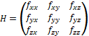
<body><![CDATA[<p style='text-align:justify'><span lang=EN-US style='font-size:10.0pt;mso-bidi-font-size:12.0pt;mso-ansi-language:EN-US'> <font face="Verdana"><![if !supportEmptyParas]>&nbsp;<![endif]></font><o:p></o:p></span></p>      <p style='text-align:justify'><span lang=EN-US style='font-size:10.0pt;mso-bidi-font-size:12.0pt;mso-ansi-language:EN-US'> <font face="Verdana"><![if !supportEmptyParas]>&nbsp;<![endif]></font><o:p></o:p></span></p>      <p align="center"> <font face="Verdana" size="2"> <a name="f1" href="/img/revistas/cleiej/v16n2/2a03f1.jpg"> Figure 1: Relationship of the classic surfaces with the Shape Index (SI) values </a> </font> </p>       <p style='text-align:justify'><span lang=EN-US style='font-size:10.0pt;mso-bidi-font-size:12.0pt;mso-ansi-language:EN-US'> <font face="Verdana"><![if !supportEmptyParas]>&nbsp;<![endif]></font><o:p></o:p></span></p>      <p style='text-align:justify'><span lang=EN-US style='font-size:10.0pt;mso-bidi-font-size:12.0pt;mso-ansi-language:EN-US'> <font face="Verdana"><![if !supportEmptyParas]>&nbsp;<![endif]></font><o:p></o:p></span></p>      <p style='text-align:justify'><span lang=EN-US style='font-size:10.0pt;mso-bidi-font-size:12.0pt;mso-ansi-language:EN-US'> <font face="Verdana">The Shape Index is computed as follows:</font><o:p></o:p></span></p>       <p align="center"> <font face="Verdana" size="2"> <a name="z1"> <img src="/img/revistas/cleiej/v16n2/2a03z1.gif"> </a> </font> </p>     <p style='text-align:justify'><span lang=EN-US style='font-size:10.0pt;mso-bidi-font-size:12.0pt;mso-ansi-language:EN-US'> <font face="Verdana"><![if !supportEmptyParas]>&nbsp;<![endif]></font><o:p></o:p></span></p>      <p style='text-align:justify'><span lang=EN-US style='font-size:10.0pt;mso-bidi-font-size:12.0pt;mso-ansi-language:EN-US'> <font face="Verdana">where <i style='mso-bidi-font-style:normal'>k</i><sub>1</sub>(<i style='mso-bidi-font-style: normal'>p</i>) and <i style='mso-bidi-font-style:normal'>k</i><sub>2</sub>(<i style='mso-bidi-font-style:normal'>p</i>) are the main curvatures at position <i style='mso-bidi-font-style:normal'>p</i>. The main curvatures are the curvatures of maximum and minimum value, and to compute them we use the formula proponed by Monga and Benayoun <a href="#r16">(16)</a>:</font><o:p></o:p></span></p>       <p align="center"> <font face="Verdana" size="2"> <a name="z2"> <img src="/img/revistas/cleiej/v16n2/2a03z2.gif"> </a> </font> </p>        ]]></body>

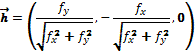
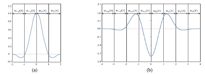
<body><![CDATA[<p style='text-align:justify'><span lang=EN-US style='font-size:10.0pt;mso-bidi-font-size:12.0pt;mso-ansi-language:EN-US'> <font face="Verdana">where</font><o:p></o:p></span></p>       <p align="center"> <font face="Verdana" size="2"> <a name="z3"> <img src="/img/revistas/cleiej/v16n2/2a03z3.gif"> </a> </font> </p>      <p align="center"> <font face="Verdana" size="2"> <a name="z4"> <img src="/img/revistas/cleiej/v16n2/2a03z4.gif"> </a> </font> </p>      <p align="center"> <font face="Verdana" size="2"> <a name="z5"> <img src="/img/revistas/cleiej/v16n2/2a03z5.gif"> </a> </font> </p>      <p style='text-align:justify'><span lang=EN-US style='font-size:10.0pt;mso-bidi-font-size:12.0pt;mso-ansi-language:EN-US'> <font face="Verdana">with <a name="z6"> <img src="/img/revistas/cleiej/v16n2/2a03z6.gif"> </a>, <a name="z7"> <img src="/img/revistas/cleiej/v16n2/2a03z7.gif"> </a>, and <a name="z8"> <img src="/img/revistas/cleiej/v16n2/2a03z8.gif"> </a>,  being <i style='mso-bidi-font-style:normal'>f</i> the function that represents the volume. In order to obtain the approximate value of the first and second degree partial derivatives at a specific point, we need to perform a convolution in that point with an appropriate convolution kernel. That kernel is built based on the method proposed by Möller et al. <a href="#r17">(17)</a>, which can be summarized in 3 steps: Build the 1D interpolation filters, discretize the filters to some number of samples, and build the 3D filters.</font><o:p></o:p></span></p>      <p style='text-align:justify'><span lang=EN-US style='font-size:10.0pt;mso-bidi-font-size:12.0pt;mso-ansi-language:EN-US'> <font face="Verdana"><![if !supportEmptyParas]>&nbsp;<![endif]></font><o:p></o:p></span></p>      <p style='margin-top:0cm;margin-right:0cm;margin-bottom:5.95pt;margin-left: 0cm;text-align:justify;text-indent:0cm;mso-pagination:none;page-break-after: auto;mso-list:none;tab-stops:35.4pt'><i style='mso-bidi-font-style:normal'> <span lang=EN-GB style='font-size:10.0pt;mso-bidi-font-size:12.0pt;font-family:"Verdana"; mso-ansi-language:EN-GB;text-decoration:none;text-underline:none'>3.2.1 </span> <span lang=EN-US style='font-size:10.0pt; mso-bidi-font-size:12.0pt;font-family:"Verdana";mso-ansi-language:EN-US; text-decoration:none;text-underline:none'>Build 1D interpolation filters</span><span lang=EN-GB style='font-size:10.0pt; mso-bidi-font-size:12.0pt;font-family:"Times New Roman";mso-ansi-language:EN-GB; text-decoration:none;text-underline:none'><o:p></o:p></span></i></p>      <p style='text-align:justify;mso-pagination:none'><font face="Verdana"><span lang=FR style='font-size:10.0pt;mso-bidi-font-size:12.0pt;mso-ansi-language: FR'>Möller et al. </span></font><span lang=EN-US style='font-size:10.0pt;mso-bidi-font-size: 12.0pt;mso-ansi-language:EN-US'><font face="Verdana"><a href="#r17">(17)</a> describe how to design interpolation filters and derivatives with a minimum numerical error. In order to do this, they use Taylor expansions for the sums of convolutions. They also established that in order to build a 1D interpolation filter, first we have to define what derivative we want to reconstruct, what precision we need in the reconstruction process, and what kind of continuity <i style='mso-bidi-font-style:normal'>C<sup>n</sup></i> we need for the reconstructed function. </font> <o:p></o:p></span></p>      <p style='text-align:justify;text-indent:18.0pt'><span lang=EN-US style='font-size:10.0pt;mso-bidi-font-size:12.0pt;mso-ansi-language: EN-US'><font face="Verdana">In our case, we need the following filters: a derivative of degree 0 (also known as an interpolation filter), a derivative of degree 1, and a derivative of degree 2. Regarding the precision, we tolerate and error of order 3 and a continuity of <i style='mso-bidi-font-style:normal'>C<sup>2</sup></i>. An equation system is obtained from the Taylor expansion series and the restrictions given by the degree of the derivative, the degree of the error, and the desired continuity. Solving this equation system produces the formula for filter <i style='mso-bidi-font-style:normal'>w</i>(<i style='mso-bidi-font-style: normal'>&#964;</i>), in several pieces <i style='mso-bidi-font-style:normal'>w<sub>k</sub></i>(<i style='mso-bidi-font-style:normal'>&#964;</i>). With and error of degree 3 and continuity <i style='mso-bidi-font-style:normal'>C</i><sup>2</sup>, the interpolation filter is defined by 4 pieces, the derivative of degree 1 is defined by 6 pieces, and the filter for derivative 2 by 8 pieces. <a href="#f2"> Figure 2</a> shows two of the obtained filters.</font><o:p></o:p></span></p>      <p style='text-align:justify;text-indent:18.0pt'><span lang=EN-US style='font-size:10.0pt;mso-bidi-font-size:12.0pt;mso-ansi-language: EN-US'><font face="Verdana">We used the 1D interpolation filter and the 1D derivative of degree 1 from Möller et al. <a href="#r17">(17)</a>. Using a similar procedure, we obtained the 1D filter for the derivative of degree 2. </font> <o:p></o:p></span></p>      ]]></body>
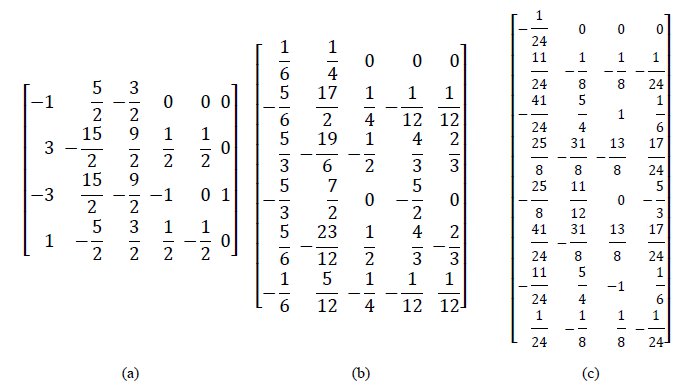
<body><![CDATA[<p align=center style='text-align:center'><span lang=EN-US style='mso-ansi-language:EN-US'><font face="Verdana" size="2"><span style="mso-spacerun: yes"> </span></font><o:p></o:p></span></p>      <p align="center"> <font face="Verdana" size="2"> <a name="f2" href="/img/revistas/cleiej/v16n2/2a03f2.jpg"> Figure 2: Filter w(&#964;) defined by 4 pieces for derivative 0 (a), and by 8 pieces for derivative 2 (b) </a> </font> </p>      <p align=center style='margin-top:5.95pt;text-align:center; text-indent:18.0pt'><span lang=EN-US style='font-size:10.0pt;mso-bidi-font-size: 12.0pt;mso-ansi-language:EN-US'><font face="Verdana"><![if !supportEmptyParas]>&nbsp;<![endif]></font><o:p></o:p></span></p>      <p style='text-align:justify;text-indent:18.0pt'><span lang=EN-US style='font-size:10.0pt;mso-bidi-font-size:12.0pt;mso-ansi-language: EN-US'><font face="Verdana"><![if !supportEmptyParas]>&nbsp;<![endif]></font><o:p></o:p></span></p>      <p style='text-align:justify;text-indent:18.0pt'><font face="Verdana"><span lang=EN-US style='font-size:10.0pt;mso-bidi-font-size:12.0pt;mso-ansi-language: EN-US'>Let [<i style='mso-bidi-font-style:normal'>w</i></span></font><sub><span style='mso-char-type:symbol;mso-symbol-font-family:Symbol; font-size:10.0pt; font-family:Verdana; mso-ascii-font-family:Times New Roman; mso-hansi-font-family:Times New Roman; mso-ansi-language:EN-US' lang="EN-US">-</span></sub><font face="Verdana"><sub><span lang=EN-US style='font-size:10.0pt;mso-bidi-font-size:12.0pt;mso-ansi-language: EN-US'>4</span></sub><span lang=EN-US style='font-size:10.0pt;mso-bidi-font-size: 12.0pt;mso-ansi-language:EN-US'>, <i style='mso-bidi-font-style:normal'>w</i></span></font><sub><span style='mso-char-type:symbol;mso-symbol-font-family:Symbol; font-size:10.0pt; font-family:Verdana; mso-ascii-font-family:Times New Roman; mso-hansi-font-family:Times New Roman; mso-ansi-language:EN-US' lang="EN-US">-</span></sub><font face="Verdana"><sub><span lang=EN-US style='font-size:10.0pt;mso-bidi-font-size:12.0pt;mso-ansi-language: EN-US'>3</span></sub><span lang=EN-US style='font-size:10.0pt;mso-bidi-font-size: 12.0pt;mso-ansi-language:EN-US'>, <i style='mso-bidi-font-style:normal'>w</i></span></font><sub><span style='mso-char-type:symbol;mso-symbol-font-family:Symbol; font-size:10.0pt; font-family:Verdana; mso-ascii-font-family:Times New Roman; mso-hansi-font-family:Times New Roman; mso-ansi-language:EN-US' lang="EN-US">-</span></sub><font face="Verdana"><sub><span lang=EN-US style='font-size:10.0pt;mso-bidi-font-size:12.0pt;mso-ansi-language: EN-US'>2</span></sub><span lang=EN-US style='font-size:10.0pt;mso-bidi-font-size: 12.0pt;mso-ansi-language:EN-US'>, <i style='mso-bidi-font-style:normal'>w</i></span></font><sub><span style='mso-char-type:symbol;mso-symbol-font-family:Symbol; font-size:10.0pt; font-family:Verdana; mso-ascii-font-family:Times New Roman; mso-hansi-font-family:Times New Roman; mso-ansi-language:EN-US' lang="EN-US">-</span></sub><font face="Verdana"><sub><span lang=EN-US style='font-size:10.0pt;mso-bidi-font-size:12.0pt;mso-ansi-language: EN-US'>1</span></sub></font><span lang=EN-US style='font-size:10.0pt;mso-bidi-font-size: 12.0pt;mso-ansi-language:EN-US'><font face="Verdana">, <i style='mso-bidi-font-style:normal'>w</i><sub>0</sub>, <i style='mso-bidi-font-style:normal'>w</i><sub>1</sub>, <i style='mso-bidi-font-style: normal'>w</i><sub>2</sub>, <i style='mso-bidi-font-style:normal'>w</i><sub>3</sub>]<i style='mso-bidi-font-style:normal'><sup>T</sup></i> =<i style='mso-bidi-font-style: normal'>M . </i>[<i style='mso-bidi-font-style:normal'>t</i><sup>3</sup>, <i style='mso-bidi-font-style:normal'>t</i><sup>2</sup>, <i style='mso-bidi-font-style: normal'>t</i>, 1]<i style='mso-bidi-font-style:normal'><sup>T</sup></i> be the general form of our 1D filters. The coefficient matrix <i style='mso-bidi-font-style: normal'>M</i> for each filter is shown in <a href="#f3"> Figure 3</a>.</font><o:p></o:p></span></p>      <p align="center"> <font face="Verdana" size="2"> <a name="f3" href="/img/revistas/cleiej/v16n2/2a03f3.jpg"> Figure 3: Coefficient matrix for each filter. (a) Interpolation filter. (b) First derivative filter. (c) Second derivative filter </a> </font> </p>      <p style='text-align:justify;text-indent:18.0pt'><span lang=EN-US style='font-size:10.0pt;mso-bidi-font-size:12.0pt;mso-ansi-language: EN-US'><font face="Verdana"><![if !supportEmptyParas]>&nbsp;<![endif]></font><o:p></o:p></span></p>      <p style='margin-top:0cm;margin-right:0cm;margin-bottom:5.95pt;margin-left: 0cm;text-align:justify;text-indent:0cm;mso-pagination:none;page-break-after: auto;mso-list:none;tab-stops:35.4pt'><i style='mso-bidi-font-style:normal'> <span lang=EN-GB style='font-size:10.0pt;mso-bidi-font-size:12.0pt;font-family:"Verdana"; mso-ansi-language:EN-GB;text-decoration:none;text-underline:none'>3.2.2 </span> <span lang=EN-US style='font-size:10.0pt; mso-bidi-font-size:12.0pt;font-family:"Verdana";mso-ansi-language:EN-US; text-decoration:none;text-underline:none'>Filter Discretization</span></i><b style='mso-bidi-font-weight:normal'><span lang=EN-US style='font-size:10.0pt; mso-bidi-font-size:12.0pt;font-family:"Times New Roman";mso-ansi-language:EN-US'><o:p></o:p></span></b></p>      <p style='text-align:justify;mso-pagination:none'><span lang=EN-US style='font-size:10.0pt;mso-bidi-font-size:12.0pt;mso-ansi-language: EN-US'><font face="Verdana">To define the filter <i style='mso-bidi-font-style:normal'>w</i>(<i style='mso-bidi-font-style:normal'>&#964;</i>) from its pieces <i style='mso-bidi-font-style:normal'>w<sub>k</sub></i>(<i style='mso-bidi-font-style: normal'>&#964;</i>), we have to consider that the support of each piece <i style='mso-bidi-font-style:normal'>w<sub>k</sub></i>(<i style='mso-bidi-font-style: normal'>&#964;</i>) is [0,1], but it represents the domain [-<i style='mso-bidi-font-style:normal'>k</i>,-<i style='mso-bidi-font-style:normal'>k</i>+1] in <i style='mso-bidi-font-style:normal'>w</i>(<i style='mso-bidi-font-style: normal'>&#964;</i>) according to <a href="#f2"> Figure 2</a>. Hence, we define <i style='mso-bidi-font-style:normal'>w<sub>k</sub></i>(<i style='mso-bidi-font-style: normal'>&#964;</i>)=<i style='mso-bidi-font-style:normal'>w</i>(<i style='mso-bidi-font-style:normal'>&#964;</i>+<i style='mso-bidi-font-style: normal'>k</i>). From the obtained filters we create the 1D kernels. For this we take equally separated samples on the domain of the filter. The samples are not taken on the borders of the filter since their value is always zero. Therefore, if we need to obtain <i style='mso-bidi-font-style:normal'>&#951;</i> samples, we must divide the filter domain in <i style='mso-bidi-font-style:normal'>&#951;</i>+1 intervals of the same size, and the samples will be taken in the points that are between two intervals. It should be noted that <i style='mso-bidi-font-style: normal'>&#951; </i>must be an odd number. In the tests that we performed we used several filters of different sizes, varying <i style='mso-bidi-font-style: normal'>&#951; </i>between 11 and 29.</font><o:p></o:p></span></p>      <p style='text-align:justify;text-indent:18.15pt'><span lang=EN-US style='font-size:10.0pt;mso-bidi-font-size:12.0pt;mso-ansi-language: EN-US'><font face="Verdana"><![if !supportEmptyParas]>&nbsp;<![endif]></font><o:p></o:p></span></p>      ]]></body>
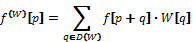
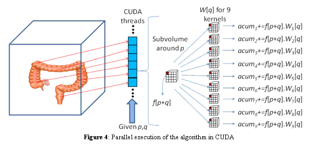
<body><![CDATA[<p style='margin-top:0cm;margin-right:0cm;margin-bottom:5.95pt;margin-left: 0cm;text-align:justify;text-indent:0cm;mso-list:none;tab-stops:35.4pt'><i style='mso-bidi-font-style:normal'> <span lang=EN-GB style='font-size:10.0pt; mso-bidi-font-size:12.0pt;font-family:"Verdana";mso-ansi-language:EN-GB; text-decoration:none;text-underline:none'>3.2.3 </span></i><i style='mso-bidi-font-style: normal'><font face="Verdana"> <span lang=EN-US style='font-size:10.0pt;mso-bidi-font-size:12.0pt; mso-ansi-language:EN-US;text-decoration:none; text-underline:none'>3D Filter Construction</span></font><o:p></o:p></i></p>      <p style='text-align:justify'><font face="Verdana"><span lang=EN-US style='font-size:10.0pt;mso-bidi-font-size:12.0pt;mso-ansi-language:EN-US'>Each of the 3D convolution kernels <i style='mso-bidi-font-style:normal'>W</i></span><i style='mso-bidi-font-style:normal'><span lang=EN-US style='font-size:10pt; font-family:"Cambria Math";mso-ansi-language:EN-US'> </span></i></font><span lang=EN-US style='font-size:10.0pt;mso-bidi-font-size:12.0pt;mso-ansi-language: EN-US'><font face="Verdana">is obtained from the following formula:</font><o:p></o:p></span></p>      <p align="center"> <font face="Verdana" size="2"> <a name="z9"> <img src="/img/revistas/cleiej/v16n2/2a03z9.gif"> </a> </font> </p>      <p style='text-align:justify'><span lang=EN-US style='font-size:10.0pt;mso-bidi-font-size:12.0pt;mso-ansi-language:EN-US'> <font face="Verdana">where <i style='mso-bidi-font-style:normal'>w<sub>x</sub></i>, <i style='mso-bidi-font-style: normal'>w<sub>y</sub></i> and <i style='mso-bidi-font-style:normal'>w<sub>z</sub></i> are the 1D kernels of the derivatives that we want to obtain in the <i style='mso-bidi-font-style:normal'>x</i>, <i style='mso-bidi-font-style:normal'>y</i> and <i style='mso-bidi-font-style:normal'>z,</i> respectively. For example, to build the kernel that approximates the value <i style='mso-bidi-font-style: normal'>&#8706;</i><sup>2</sup><i style='mso-bidi-font-style:normal'>f</i>/<i style='mso-bidi-font-style:normal'>&#8706;x</i><sup>2</sup>, <i style='mso-bidi-font-style:normal'>w<sub>x</sub></i> would have the values obtained for the 1D kernel of the second degree derivative, while <i style='mso-bidi-font-style:normal'>w<sub>y</sub></i> and <i style='mso-bidi-font-style: normal'>w<sub>z</sub></i> would have the values obtained by the 1D interpolation kernel (derivative of degree 0). In order to approximate all the required partial derivatives, 9 convolution kernels are built, 3 for the first degree partial derivatives: &#8706;<i style='mso-bidi-font-style:normal'>f</i>/&#8706;<i style='mso-bidi-font-style:normal'>x</i>, &#8706;<i style='mso-bidi-font-style: normal'>f</i>/&#8706;<i style='mso-bidi-font-style:normal'>y</i>, &#8706;<i style='mso-bidi-font-style:normal'>f</i>/&#8706;<i style='mso-bidi-font-style: normal'>z</i>; and other 6 for the second order partial derivatives: <i style='mso-bidi-font-style:normal'>&#8706;</i><sup>2</sup><i style='mso-bidi-font-style: normal'>f</i>/<i style='mso-bidi-font-style:normal'>&#8706;x</i><sup>2</sup>, &#8706;<sup>2</sup><i style='mso-bidi-font-style:normal'>f</i>/&#8706;<i style='mso-bidi-font-style:normal'>y</i><sup>2</sup>, <i style='mso-bidi-font-style: normal'>&#8706;f</i><sup>2</sup>/<i style='mso-bidi-font-style:normal'>&#8706;z</i><sup>2</sup>, <i style='mso-bidi-font-style:normal'>&#8706;</i><sup>2</sup><i style='mso-bidi-font-style:normal'>f</i>/(<i style='mso-bidi-font-style:normal'>&#8706;x&#8706;y</i>), <i style='mso-bidi-font-style:normal'>&#8706;</i><sup>2</sup><i style='mso-bidi-font-style:normal'>f</i>/(<i style='mso-bidi-font-style:normal'>&#8706;x&#8706;z</i>), &#8706;<sup>2</sup><i style='mso-bidi-font-style:normal'>f</i>/(<i style='mso-bidi-font-style:normal'>&#8706;y&#8706;z</i>).</font><o:p></o:p></span></p>      <p style='text-align:justify;text-indent:18.0pt'><font face="Verdana"><span lang=EN-US style='font-size:10.0pt;mso-bidi-font-size:12.0pt;mso-ansi-language: EN-US'>Once the convolution kernels are obtained, the values of the first and second order partial derivatives in the points on the surface of the colon wall are approximated. Let <i style='mso-bidi-font-style:normal'>C</i> be an array storing that set of points, and assuming that the central position of a filter <i style='mso-bidi-font-style:normal'>W</i> is point (0,0,0), the value of the convolution in the point <i style='mso-bidi-font-style:normal'>p</i></span><span lang=EN-US style='mso-ansi-language:EN-US'><font size="2"> </font> </span><span lang=EN-US style='font-size:10.0pt;mso-bidi-font-size:12.0pt;mso-ansi-language:EN-US'>in</span><span lang=EN-US style='mso-ansi-language:EN-US'><font size="2"> </font> </span><i style='mso-bidi-font-style: normal'><span lang=EN-US style='font-size:10.0pt;mso-bidi-font-size:12.0pt; mso-ansi-language:EN-US'>C</span></i></font><span lang=EN-US style='font-size:10.0pt; mso-bidi-font-size:12.0pt;mso-ansi-language:EN-US'><font face="Verdana"> is given by the formula:</font><o:p></o:p></span></p>      <p align="center"> <font face="Verdana" size="2"> <a name="z10"> <img src="/img/revistas/cleiej/v16n2/2a03z10.gif"> </a> </font> </p>       <p style='text-align:justify'> <span lang=EN-US style='font-size:10.0pt;mso-bidi-font-size:12.0pt;mso-ansi-language:EN-US'> <font face="Verdana">where  <a name="z11"> <img src="/img/revistas/cleiej/v16n2/2a03z11.gif"> </a>  is the value of the partial derivative in <i style='mso-bidi-font-style: normal'>p </i>approximated by the convolution kernel <i style='mso-bidi-font-style: normal'>W</i>. Those <i style='mso-bidi-font-style:normal'>p</i>+<i style='mso-bidi-font-style:normal'>q</i> values out of the volume are clamped to the volume border. This is done in order to avoid any abrupt cut, because this could produce incorrect polyp detections.</font><o:p></o:p></span></p>      <p style='text-align:justify;text-indent:18.15pt'><span lang=EN-US style='font-size:10.0pt;mso-bidi-font-size:12.0pt;mso-ansi-language: EN-US'><font face="Verdana">Computing the convolution for all points <i style='mso-bidi-font-style: normal'>p</i> in<i style='mso-bidi-font-style:normal'> C</i> is a process that requires intensive computing. For this reason, this part of the method is implemented using parallel programming in CUDA, whereby multiple threads can be executed in multiple CUDA processing cores. The general idea is to have multiple threads execute the same instructions for different data. If the execution time of threads was unlimited, each thread could compute different convolutions of a <i style='mso-bidi-font-style:normal'>p</i> in<i style='mso-bidi-font-style:normal'> C. </i>However, there are restrictions on the executing time of threads, so the computation assigned to each thread is just a term on the sum of the convolution for a <i style='mso-bidi-font-style: normal'>p</i> in<i style='mso-bidi-font-style:normal'> C.</i> On each thread activation, a term is computed, and the partial sum with that term is updated. In order to avoid consistency problems, the threads must be synchronized before computing each term of the sum. This process is repeated until all the terms of the convolution are computed.</font><o:p></o:p></span></p>      <p style='text-align:justify;text-indent:18.15pt'><span lang=EN-US style='font-size:10.0pt;mso-bidi-font-size:12.0pt;mso-ansi-language: EN-US'><font face="Verdana">In order to reduce the amount of synchronizations, each thread computes one term of each of the 9 convolutions which must be done for each point. This way, each thread activation performs 9 computations of the form: </font> <o:p></o:p></span></p>      <p align="center"> <font face="Verdana" size="2"> <a name="z12"> <img src="/img/revistas/cleiej/v16n2/2a03z12.gif"> </a> </font> </p>      ]]></body>

<body><![CDATA[<p style='text-align:justify'><font face="Verdana"><span lang=EN-US style='font-size:10.0pt;mso-bidi-font-size:12.0pt;mso-ansi-language:EN-US'>where <i style='mso-bidi-font-style:normal'>p</i> represents the position (<i style='mso-bidi-font-style:normal'>x</i>,<i style='mso-bidi-font-style:normal'>y</i>,<i style='mso-bidi-font-style:normal'>z</i>) of a voxel of the colon wall in the volume, and <i style='mso-bidi-font-style:normal'>q</i> represents a translation (<i style='mso-bidi-font-style:normal'>dx</i>,<i style='mso-bidi-font-style: normal'>dy</i>,<i style='mso-bidi-font-style:normal'>dz</i>) necessary to compute a term of the convolution between the voxel <i style='mso-bidi-font-style: normal'>p</i> and the filter <i style='mso-bidi-font-style:normal'>W</i> centered on <i style='mso-bidi-font-style:normal'>p</i> (see <a href="#f4"> Figure 4</a>). Each CUDA thread receives a position <i style='mso-bidi-font-style:normal'>p</i> in <i style='mso-bidi-font-style:normal'>C</i> and a translation <i style='mso-bidi-font-style: normal'>q</i> in the convolution filters. A thread computes the convolution term <i style='mso-bidi-font-style:normal'>f</i>[<i style='mso-bidi-font-style: normal'>p</i>+<i style='mso-bidi-font-style:normal'>q</i>].<i style='mso-bidi-font-style: normal'>W</i>[<i style='mso-bidi-font-style:normal'>q</i>] for 9 filters <i style='mso-bidi-font-style:normal'>W</i>, so it performs 9 multiplications. On every execution of a thread, it accumulates that term in its accumulator (<i style='mso-bidi-font-style:normal'>acum</i>), which is equivalent to performing 9 sums. When all the threads that compute a term of the convolution end their execution, the execution of the threads that will compute the next term starts. When all terms have been computed and accumulated on the threads, another group of positions <i style='mso-bidi-font-style:normal'>p </i>in<i style='mso-bidi-font-style: normal'> C</i> is processed, until all the entries in <i style='mso-bidi-font-style: normal'>C</i> have been processed.</span></font><span lang=EN-US style='font-size: 10.0pt;mso-ansi-language:EN-US;mso-fareast-language:ES-VE'><o:p></o:p></span></p>      <p style='text-align:justify;mso-pagination:none'><span lang=EN-US style='font-size:10.0pt;mso-ansi-language:EN-US'> <font face="Verdana"><![if !supportEmptyParas]>&nbsp;<![endif]></font><o:p></o:p></span></p>      <p align="center"> <font face="Verdana" size="2"> <a name="f4" href="/img/revistas/cleiej/v16n2/2a03f4.gif"> Figure 4: Parallel execution of the algorithm in CUDA </a> </font> </p>      <p style='text-align:justify;mso-pagination:none'><span lang=EN-US style='font-size:10.0pt;mso-ansi-language:EN-US'> <font face="Verdana"><![if !supportEmptyParas]>&nbsp;<![endif]></font><o:p></o:p></span></p>      <p style='margin-top:0cm;margin-right:0cm;margin-bottom:5.95pt;margin-left: 0cm;text-align:justify;text-indent:0cm;mso-pagination:none;page-break-after: auto;mso-list:none;tab-stops:35.4pt'><font face="Verdana"> <span lang=EN-US style='font-size:10.0pt; mso-bidi-font-size:12.0pt;mso-ansi-language:EN-US'>3.3 Candidate Selection and Grouping</span></font><o:p></o:p></p>      <p style='text-align:justify;mso-pagination:none'><font face="Verdana"><span lang=EN-US style='font-size:10.0pt;mso-bidi-font-size:12.0pt;mso-ansi-language: EN-US'>Usually, the top part of a polyp looks like a cup. Therefore we need to select voxels whose neighborhood has a likely shape. As can be seen in Fig</span><span lang=EN-US style='font-size:10.0pt;mso-ansi-language:EN-US'>ure 1, if the value of <i style='mso-bidi-font-style:normal'>SI</i> is close to 1.0, the surface near this point presents a shape similar to the desired shape. Empirically, we set that a voxel can belong to a polyp if <i style='mso-bidi-font-style:normal'>SI</i> &gt; 0.85. Voxels <i style='mso-bidi-font-style:normal'>v</i> satisfying this condition are stored in an array we call <i style='mso-bidi-font-style:normal'>S</i>. Based on tests done by </span></font><span lang=EN-US style='font-size:10.0pt; mso-bidi-font-size:12.0pt;mso-ansi-language:EN-US'><font face="Verdana">Yoshida and Nappi <a href="#r3">(3)</a>, voxel candidates usually gather on top of polyps. Hence, we can group voxel candidates by their proximity, considering that they can be part of the same polyp or structure. In order to accomplish the grouping, a 3D boolean array <i style='mso-bidi-font-style:normal'>B</i> with the same dimensions of the original volume was created, and the positions of the selected points are marked. The algorithm for grouping voxels is the following:</font><o:p></o:p></span></p>      <p style='text-align:justify;tab-stops:166.55pt'><span lang=EN-US style='font-size:10.0pt;mso-bidi-font-size:12.0pt;mso-ansi-language: EN-US'><font face="Verdana"><span style='mso-tab-count:1'>                                                                          </span> </font><o:p></o:p></span></p>      <p style='text-align:justify;tab-stops:166.55pt'><span lang=EN-US style='font-size:10.0pt;mso-bidi-font-size:12.0pt;mso-ansi-language: EN-US'><font face="Verdana"><![if !supportEmptyParas]>&nbsp;<![endif]></font><o:p></o:p></span></p>      <p style='margin-left:54.15pt;text-indent:-18.0pt; mso-list:l7 level1 lfo8'><![if !supportLists]><span lang=EN-US style='font-size:10.0pt;mso-ansi-language:EN-US'><font face="Verdana">1.</font><span style='font-style:normal; font-variant:normal; font-weight:normal; font-family:Verdana'>&nbsp;&nbsp;&nbsp;&nbsp;&nbsp;&nbsp;&nbsp; </span></span><![endif]><span lang=EN-US style='font-size:10.0pt;mso-ansi-language: EN-US'><font face="Verdana">Create an empty group <i style='mso-bidi-font-style:normal'>G</i> and an empty auxiliary queue <i style='mso-bidi-font-style:normal'>Q</i>.</font><o:p></o:p></span></p>      <p style='margin-left:54.15pt;text-indent:-18.0pt; mso-list:l7 level1 lfo8'><![if !supportLists]><span lang=EN-US style='font-size:10.0pt;mso-ansi-language:EN-US'><font face="Verdana">2.</font><span style='font-style:normal; font-variant:normal; font-weight:normal; font-family:Verdana'>&nbsp;&nbsp;&nbsp;&nbsp;&nbsp;&nbsp;&nbsp; </span></span><![endif]><span lang=EN-US style='font-size:10.0pt;mso-ansi-language: EN-US'><font face="Verdana">Move any given voxel from <i style='mso-bidi-font-style:normal'>S</i> to <i style='mso-bidi-font-style:normal'>Q</i>, and unmark it as selected in <i style='mso-bidi-font-style:normal'>B</i>.</font><o:p></o:p></span></p>      ]]></body>
<body><![CDATA[<p style='margin-left:54.15pt;text-indent:-18.0pt; mso-list:l7 level1 lfo8'><![if !supportLists]><span lang=EN-US style='font-size:10.0pt;mso-ansi-language:EN-US'><font face="Verdana">3.</font><span style='font-style:normal; font-variant:normal; font-weight:normal; font-family:Verdana'>&nbsp;&nbsp;&nbsp;&nbsp;&nbsp;&nbsp;&nbsp; </span></span><![endif]><span lang=EN-US style='font-size:10.0pt;mso-ansi-language: EN-US'><font face="Verdana">Extract a voxel <i style='mso-bidi-font-style:normal'>v</i> from <i style='mso-bidi-font-style:normal'>Q</i>, and add it to group <i style='mso-bidi-font-style:normal'>G</i>.</font><o:p></o:p></span></p>      <p style='margin-left:54.15pt;text-indent:-18.0pt; mso-list:l7 level1 lfo8'><![if !supportLists]><span lang=EN-US style='font-size:10.0pt;mso-ansi-language:EN-US'><font face="Verdana">4.</font><span style='font-style:normal; font-variant:normal; font-weight:normal; font-family:Verdana'>&nbsp;&nbsp;&nbsp;&nbsp;&nbsp;&nbsp;&nbsp; </span></span><![endif]><span lang=EN-US style='font-size:10.0pt;mso-ansi-language: EN-US'><font face="Verdana">Check in a cubic region around <i style='mso-bidi-font-style:normal'>v</i> for other nearby voxel which are selected as well as marked in <i style='mso-bidi-font-style:normal'>B</i>.</font><o:p></o:p></span></p>      <p style='margin-left:54.15pt;text-indent:-18.0pt; mso-list:l7 level1 lfo8'><![if !supportLists]><span lang=EN-US style='font-size:10.0pt;mso-ansi-language:EN-US'><font face="Verdana">5.</font><span style='font-style:normal; font-variant:normal; font-weight:normal; font-family:Verdana'>&nbsp;&nbsp;&nbsp;&nbsp;&nbsp;&nbsp;&nbsp; </span></span><![endif]><span lang=EN-US style='font-size:10.0pt;mso-ansi-language: EN-US'><font face="Verdana">If such voxels are found, insert them in <i style='mso-bidi-font-style: normal'>Q</i>, delete them from <i style='mso-bidi-font-style:normal'>S</i>, and unmarked them in <i style='mso-bidi-font-style:normal'>B</i>.</font><o:p></o:p></span></p>      <p style='margin-left:54.15pt;text-indent:-18.0pt; mso-list:l7 level1 lfo8'><![if !supportLists]><span lang=EN-US style='font-size:10.0pt;mso-ansi-language:EN-US'><font face="Verdana">6.</font><span style='font-style:normal; font-variant:normal; font-weight:normal; font-family:Verdana'>&nbsp;&nbsp;&nbsp;&nbsp;&nbsp;&nbsp;&nbsp; </span></span><![endif]><span lang=EN-US style='font-size:10.0pt;mso-ansi-language: EN-US'><font face="Verdana">If there are voxels still left in <i style='mso-bidi-font-style:normal'>Q</i>, return to step 3.</font><o:p></o:p></span></p>      <p style='margin-left:54.15pt;text-indent:-18.0pt; mso-list:l7 level1 lfo8'><![if !supportLists]><span lang=EN-US style='font-size:10.0pt;mso-ansi-language:EN-US'><font face="Verdana">7.</font><span style='font-style:normal; font-variant:normal; font-weight:normal; font-family:Verdana'>&nbsp;&nbsp;&nbsp;&nbsp;&nbsp;&nbsp;&nbsp; </span></span><![endif]><span lang=EN-US style='font-size:10.0pt;mso-ansi-language: EN-US'><font face="Verdana">If no voxel remains in <i style='mso-bidi-font-style:normal'>Q</i>, group <i style='mso-bidi-font-style:normal'>G</i> is considered a polyp candidate, and therefore it is stored in a list of groups <i style='mso-bidi-font-style: normal'>LG</i>.</font><o:p></o:p></span></p>      <p style='margin-left:54.15pt;text-indent:-18.0pt; mso-list:l7 level1 lfo8'><![if !supportLists]><span lang=EN-US style='font-size:10.0pt;mso-ansi-language:EN-US'><font face="Verdana">8.</font><span style='font-style:normal; font-variant:normal; font-weight:normal; font-family:Verdana'>&nbsp;&nbsp;&nbsp;&nbsp;&nbsp;&nbsp;&nbsp; </span></span><![endif]><span lang=EN-US style='font-size:10.0pt;mso-ansi-language: EN-US'><font face="Verdana">If there are voxel remaining in <i style='mso-bidi-font-style:normal'>S</i>, return to step 1.</font><o:p></o:p></span></p>      <p style='text-align:justify;text-indent:18.15pt'><span lang=EN-US style='font-size:10.0pt;mso-bidi-font-size:12.0pt;mso-ansi-language: EN-US'><font face="Verdana"><![if !supportEmptyParas]>&nbsp;<![endif]></font><o:p></o:p></span></p>      <p style='text-align:justify;text-indent:18.15pt'><span lang=EN-US style='font-size:10.0pt;mso-bidi-font-size:12.0pt;mso-ansi-language: EN-US'><font face="Verdana">Each of the obtained groups in <i style='mso-bidi-font-style:normal'>LG</i> will be considered a polyp candidate. However, it is necessary to employ an additional technique to verify that in fact the voxels associated to the group are part of a structure with the shape of a polyp. For this, we defined a heuristic for determining whether the group is a good polyp candidate or not, by studying the shape of a planar cut of the candidate.</font><o:p></o:p></span></p>      <p style='text-align:justify'><span lang=EN-US style='font-size:10.0pt;mso-bidi-font-size:12.0pt;mso-ansi-language:EN-US'> <font face="Verdana"><![if !supportEmptyParas]>&nbsp;<![endif]></font><o:p></o:p></span></p>      <p style='margin-top:0cm;margin-right:0cm;margin-bottom:5.95pt;margin-left: 0cm;text-align:justify;text-indent:0cm;mso-list:none;tab-stops:35.4pt'> <font face="Verdana"> <span lang=EN-US style='font-size:10.0pt;mso-bidi-font-size:12.0pt;mso-ansi-language:EN-US'>3.4 Planar Cut Extraction</span></font><o:p></o:p></p>      ]]></body>
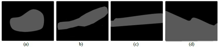
<body><![CDATA[<p style='text-align:justify'><span lang=EN-US style='font-size:10.0pt;mso-bidi-font-size:12.0pt;mso-ansi-language:EN-US'> <font face="Verdana">Each polyp candidate has a group of voxels associated to it, which we suppose are located in the top of the polyp. Assuming so, then the volumetric center <i style='mso-bidi-font-style:normal'>P</i><sub>0</sub> of these voxels must be located inside the polyp. Additionally, if we compute a normalized vector <i style='mso-bidi-font-style:normal'>N</i> corresponding to the average normal to the voxels in the same group, and we locate its origin at <i style='mso-bidi-font-style: normal'>P</i><sub>0</sub>, then we can suppose that <i style='mso-bidi-font-style: normal'>N</i> points towards the top of the polyp. Using <i style='mso-bidi-font-style: normal'>N</i> and <i style='mso-bidi-font-style:normal'>P</i><sub>0 </sub>we can construct the equation of a plane (<i style='mso-bidi-font-style:normal'>P</i>-<i style='mso-bidi-font-style:normal'>P</i><sub>0</sub>)&#903;<i style='mso-bidi-font-style: normal'>N</i>=0, which then allows us to capture an image corresponding to a planar cut of the polyp candidate (see <a href="#f5"> Figure 5</a>), so that we can study its shape later on.</font><o:p></o:p></span></p>      <p style='text-align:justify'><span lang=EN-US style='font-size:10.0pt;mso-bidi-font-size:12.0pt;mso-ansi-language:EN-US'> <font face="Verdana"><![if !supportEmptyParas]>&nbsp;<![endif]></font><o:p></o:p></span></p>      <p style='margin-top:0cm;margin-right:0cm;margin-bottom:5.95pt;margin-left: 0cm;text-align:justify;text-indent:0cm;mso-list:none;tab-stops:35.4pt'> <font face="Verdana"> <span lang=EN-US style='font-size:10.0pt;mso-bidi-font-size:12.0pt;mso-ansi-language:EN-US'>3.5 Selective Analysis</span></font><o:p></o:p></p>      <p style='text-align:justify'><span lang=EN-US style='font-size:10.0pt;mso-bidi-font-size:12.0pt;mso-ansi-language:EN-US'> <font face="Verdana">After obtaining the image of the planar cut we analyze it for selecting strong polyp candidates and discard possible false positives. It is expected that the image would contain an isolated figure, that is, a region with grey intensities (corresponding to tissue) completely surrounded by a region with dark intensities (corresponding to air). If this does not occur, most likely the grey region would intersect the border of the image, indicating that is unlikely that the candidate is a polyp. In this case, the candidate is discarded (see <a href="#f6"> Figure 6</a>). For detecting isolated figures, we use a region-growing algorithm seeded in the center of the image <i style='mso-bidi-font-style: normal'>P</i><sub>0</sub>, with an appropriate threshold.</font><o:p></o:p></span></p>      <p style='text-align:justify;text-indent:18.15pt'><span lang=EN-US style='font-size:10.0pt;mso-bidi-font-size:12.0pt;mso-ansi-language: EN-US'><font face="Verdana"><![if !supportEmptyParas]>&nbsp;<![endif]></font><o:p></o:p></span></p>      <p align="center"> <font face="Verdana" size="2"> <a name="f5" href="/img/revistas/cleiej/v16n2/2a03f5.gif"> Figure  5: Planar cut of the polyp candidate </a> </font> </p>      <p style='text-align:justify'><span lang=EN-US style='font-size:10.0pt;mso-bidi-font-size:12.0pt;mso-ansi-language:EN-US'> <font face="Verdana">Even if an isolated figure is found, if the shape of the grey region is too elongated then it is unlikely to correspond to a good candidate (see Figure 6b). For discarding such candidates we consider the relation <i style='mso-bidi-font-style:normal'>R</i> between the region’s perimeter <i style='mso-bidi-font-style:normal'>p</i> and area <i style='mso-bidi-font-style: normal'>A</i>: <span style="mso-spacerun: yes"> </span> <a name="z13"> <img src="/img/revistas/cleiej/v16n2/2a03z13.gif"> </a>, which indicates how elongated is the region. For instance, for a circle <a name="z14"> <img src="/img/revistas/cleiej/v16n2/2a03z14.gif"> </a>; for a square <i style='mso-bidi-font-style:normal'>R</i>(<i style='mso-bidi-font-style: normal'>p</i>, <i style='mso-bidi-font-style:normal'>A</i>)=16; and for a rectangle with longest side <i style='mso-bidi-font-style:normal'>L</i>=9 and shortest side <i style='mso-bidi-font-style:normal'>l</i>=1, <i style='mso-bidi-font-style:normal'>R</i>(<i style='mso-bidi-font-style:normal'>p</i>, <i style='mso-bidi-font-style:normal'>A</i>)=40. Note that the higher the value of <i style='mso-bidi-font-style:normal'>R</i> the longest is the figure. Therefore, we could use this criterion for discarding candidates with elongated shapes.</font><o:p></o:p></span></p>      <p style='text-align:justify;text-indent:18.15pt'><span lang=EN-US style='font-size:10.0pt;mso-bidi-font-size:12.0pt;mso-ansi-language: EN-US'><font face="Verdana"><![if !supportEmptyParas]>&nbsp;<![endif]></font><o:p></o:p></span></p>      <p align="center"> <font face="Verdana" size="2"> <a name="f6" href="/img/revistas/cleiej/v16n2/2a03f6.jpg"> Figure  6: Analysis of the planar cut. (a) Strong polyp candidate. (b) The region presents an elongated shape, so the candidate is discarded. In (c) and (d), the candidate is discarded since the grey region intersects the image border </a> </font> </p>      <p style='margin-left:0cm;text-align:justify;text-indent:0cm'><![if !supportLists]> <span style='font-style:normal; font-variant:normal; font-weight:normal; font-size:10pt; font-family:Verdana; mso-ansi-language:EN-US' lang="EN-US">&nbsp;&nbsp;&nbsp;&nbsp;&nbsp;&nbsp;&nbsp;&nbsp;&nbsp;&nbsp;&nbsp;&nbsp;&nbsp;&nbsp; </span><![endif]> <span lang=EN-US style='font-size:10.0pt;mso-bidi-font-size: 12.0pt;font-family:"Verdana";font-variant:normal;mso-ansi-language: EN-US'>For computing the perimeter of the region found in the planar cut, we simply count the number of pixels in the border of the region. For computing the area, we count the number of pixels inside the region. Following this, those candidates with a value of <i style='mso-bidi-font-style:normal'>R</i> higher that a certain threshold, are discarded. After the analysis, the remaining candi</span><font face="Verdana"><span lang=EN-US style='font-size:10.0pt;font-variant:normal;mso-ansi-language:EN-US'>dates are considered strong polyp candidates.</span></font><o:p></o:p></p>      ]]></body>
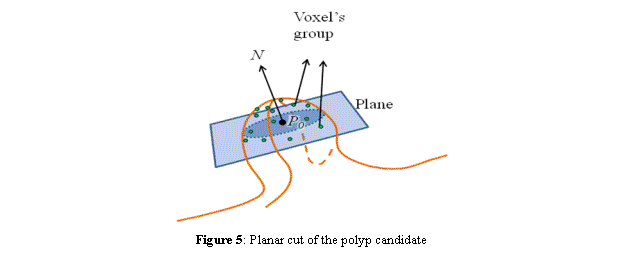

<body><![CDATA[<p style='margin-left:0cm;text-align:justify;text-indent:0cm'><![if !supportLists]> <span style='font-style:normal; font-variant:normal; font-weight:normal; font-size:10pt; font-family:Verdana; text-transform:uppercase; mso-ansi-language:EN-US' lang="EN-US">&nbsp;&nbsp;&nbsp;&nbsp;&nbsp;&nbsp;&nbsp;&nbsp;&nbsp;&nbsp;&nbsp;&nbsp;&nbsp;&nbsp; </span><![endif]> <span style="mso-spacerun: yes; font-size:10.0pt; font-variant:normal; mso-ansi-language:EN-US" lang="EN-US"> <font face="Verdana"> </font></span><span style='text-transform:uppercase'><o:p></o:p></span></p>      <p style='margin-top:0cm;margin-right:0cm;margin-bottom:5.95pt;margin-left: 0cm;text-align:justify;text-indent:0cm;mso-list:none;tab-stops:35.4pt'><b style='mso-bidi-font-weight:normal'><font face="Verdana"> <span lang=EN-US style='font-size:10pt; font-variant:normal;mso-ansi-language:EN-US'>4 Test and Results</span></font><o:p></o:p></b></p>      <p style='margin-left:0cm;text-align:justify;text-indent:0cm;mso-list:none; tab-stops:35.4pt'><font face="Verdana"> <span lang=EN-US style='font-size:10.0pt;mso-bidi-font-size: 12.0pt;font-variant:normal;mso-ansi-language: EN-US'>The main goal of the tests was counting the number of false positives removed by the selective analysis heuristic, and comparing the response times between a sequential algorithm for CPU and the parallel algorithm for GPU presented in this paper. Six CT Colonography datasets were employed for the tests. <a href="#t1"> Table 1</a> shows the characteristics of the test datasets along with the results of the first test for counting the number of detected candidates and the number of false positives removed.</span></font><o:p></o:p></p>      <p style='text-align:justify;text-indent:18.15pt'><span lang=EN-US style='font-size:10.0pt;mso-bidi-font-size:12.0pt;mso-ansi-language: EN-US'><font face="Verdana">Several key parameters were set for the first test. For the region-growing algorithm which separates the tissue from the air during the planar-cut analysis, we set a threshold of 45 for processing datasets 2, 3, 4, 5 and 6. For dataset 1 we set the threshold to 950 since it has a wider dynamic range and higher intensity values than the other datasets. For studding the shape of the tissue region, a threshold of <span style="mso-spacerun: yes"> </span>R<sub>(p,A)</sub> &gt;30 was set. </font> <o:p></o:p></span></p>      <p style='text-align:justify;text-indent:18.15pt'><font face="Verdana"><span lang=EN-US style='font-size:10.0pt;mso-bidi-font-size:12.0pt;mso-ansi-language: EN-US'>Initially, we varied the size of the convolution filters for the derivative approximation (the </span></font> <span style='mso-char-type:symbol; mso-symbol-font-family:Symbol; font-size:10.0pt; mso-bidi-font-size:12.0pt; font-family:Verdana; mso-ascii-font-family:Times New Roman; mso-hansi-font-family:Times New Roman; mso-ansi-language:EN-US' lang="EN-US">h</span><span lang=EN-US style='font-size:10.0pt;mso-bidi-font-size:12.0pt;mso-ansi-language:EN-US'><font face="Verdana"> parameter) between 11<sup>3</sup> and 29<sup>3</sup> samples, in order to find the most appropriate size for the tests datasets, and then we found that the size of the kernels affected considerably the size of the detected candidates. Moreover, we noted that setting the kernel size to 13<sup>3</sup> and 21<sup>3 </sup>was enough to detect polyp candidates of different sizes. Therefore, the kernel size was set to these two values for the first test, see column <i style='mso-bidi-font-style:normal'>kernel size</i> in <a href="#t1"> Table 1</a>. Nevertheless, it was expected that with these settings, in many cases we were going to detect the same region with both kernel sizes. Therefore, we also computed the number of detected candidates combining both kernel sizes, but eliminating repeated detections, see the last column of <a href="#t1"> Table 1</a>. This table also shows the amount of detected candidates (see column <i style='mso-bidi-font-style:normal'>detections</i>) which ranges from 249 to 760, although the majority of them are later on discarded by the planar cut analysis (see column <i style='mso-bidi-font-style: normal'>false</i> <i style='mso-bidi-font-style:normal'>positives</i>). </font> <o:p></o:p></span></p>       <p align="center"> <font face="Verdana" size="2"> <a name="t1" href="/img/revistas/cleiej/v16n2/2a03t1.jpg"> Table 1: Test datasets and results for the first test </a> </font> </p>       <p style='margin-left:0cm;text-align:justify;text-indent:0cm'><![if !supportLists]> <span style='font-style:normal; font-variant:normal; font-weight:normal; font-size:10pt; font-family:Verdana; mso-bidi-font-size:12.0pt; mso-ansi-language:EN-US' lang="EN-US">&nbsp;&nbsp;&nbsp;&nbsp;&nbsp;&nbsp;&nbsp;&nbsp;&nbsp;&nbsp;&nbsp;&nbsp;&nbsp;&nbsp; </span><![endif]> <span lang=EN-US style='font-size:10.0pt;mso-bidi-font-size: 12.0pt;font-variant:normal;mso-ansi-language: EN-US'><![if !supportEmptyParas]><font face="Verdana">&nbsp;</font><![endif]></span><o:p></o:p></p>      <p style='text-align:justify;text-indent:18.15pt'><span lang=EN-US style='font-size:10.0pt;mso-bidi-font-size:12.0pt;mso-ansi-language: EN-US'><font face="Verdana">From all datasets, we only had a medical report for datasets 5 and 6. These two datasets were acquired from the same patient. Dataset 5 was acquired in prone position and dataset 6 in supine position. They were both obtained from <a href="#r18">(18)</a> along with their medical reports. For these two datasets, all the polyps mentioned in the medical reports were detected by our approach. <a href="#f7"> Figure 7</a> shows screenshots of the detected polyps, along with a few false positives.</font><o:p></o:p></span></p>      <p style='text-align:justify;text-indent:18.15pt'><span lang=EN-US style='font-size:10.0pt;mso-bidi-font-size:12.0pt;mso-ansi-language: EN-US'><font face="Verdana"><![if !supportEmptyParas]>&nbsp;<![endif]></font><o:p></o:p></span></p>      <p align="center"> <font face="Verdana" size="2"> <a name="f7" href="/img/revistas/cleiej/v16n2/2a03f7.jpg"> Figure  7: Polyp candidates obtained from datasets 5 and 6. (a) Real polyps diagnosed by a medical doctor. (b,c) False positives </a> </font> </p>      ]]></body>
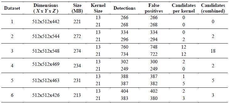
<body><![CDATA[<p style='text-align:justify;text-indent:18.15pt'><span lang=EN-US style='font-size:10.0pt;mso-bidi-font-size:12.0pt;mso-ansi-language: EN-US'><font face="Verdana"><![if !supportEmptyParas]>&nbsp;<![endif]></font><o:p></o:p></span></p>      <p style='margin-left:0cm;text-align:justify;text-indent:0cm'><![if !supportLists]> <span style='font-style:normal; font-variant:normal; font-weight:normal; font-size:10pt; font-family:Verdana; mso-bidi-font-size:12.0pt; mso-ansi-language:EN-US' lang="EN-US">&nbsp;&nbsp;&nbsp;&nbsp;&nbsp;&nbsp;&nbsp;&nbsp;&nbsp;&nbsp;&nbsp;&nbsp;&nbsp;&nbsp; </span><![endif]><font face="Verdana"> <span lang=EN-US style='font-size:10.0pt;mso-bidi-font-size: 12.0pt;font-variant:normal;mso-ansi-language: EN-US'>We also performed an <i style='mso-bidi-font-style:normal'>electronic biopsy</i> <a href="#r19">(19)</a> on the two diagnosed polyps in datasets 5 and 6. The technique consists of producing a translucent version of the VC images by mapping the intensity values in the original data to different colors and opacities, in such a way that the interior structure of the polyps can be visible. In the translucent image the interior of metaplastic polyps looks different than the interior of adenomatous polyps. <a href="#f8"> Figure 8</a> shows the electronic biopsy for the two diagnosed polyps in <a href="#f7"> Figure 7</a>a.</span></font><o:p></o:p></p>      <p style='text-align:justify;text-indent:21.3pt'><span lang=EN-US style='font-size:10.0pt;mso-bidi-font-size:12.0pt;mso-ansi-language: EN-US'><font face="Verdana">Figure 9 shows screenshots for some of the detections in datasets 1, 2, 3 and 4. Notice that all of them have the typical shape of a polyp. However, we did not have a medical report for these datasets. Therefore, we could only employ the electronic biopsy technique to rule out false detections in these results. <a href="#f10"> Figure 10</a> shows the electronic biopsy technique being applied on the three polyps at the bottom of Figure 9. Notice that <a href="#f10">Figure 10</a>b looks different than the others, because this detection actually corresponds to a residual stool ball, not to a polyp. Figures 10a y 10c look similar to the images in <a href="#f8"> Figure 8</a>, but we did not have any medical report to prove that these are real polyps. Therefore, it was impossible for us to calculate the actual accuracy of our method.</font><o:p></o:p></span></p>      <p style='text-align:justify;text-indent:21.3pt'><span lang=EN-US style='font-size:10.0pt;mso-bidi-font-size:12.0pt;mso-ansi-language: EN-US'><font face="Verdana"><![if !supportEmptyParas]>&nbsp;<![endif]></font><o:p></o:p></span></p>      <p align="center"> <font face="Verdana" size="2"> <a name="f8" href="/img/revistas/cleiej/v16n2/2a03f8.jpg"> Figure  8: Electronic biopsy of two polyps diagnosed by a medical doctor in datasets 5 and 6. Both polyps appear to be adenomatous polyps </a> </font> </p>      <p align="center"> <font face="Verdana" size="2"> <a name="f9" href="/img/revistas/cleiej/v16n2/2a03f9.jpg"> Figure  9: Polyp candidate examples obtained from datasets 1, 2, 3 and 4 </a> </font> </p>      <p align="center"> <font face="Verdana" size="2"> <a name="f10" href="/img/revistas/cleiej/v16n2/2a03f10.jpg"> Figure  10: Polyp candidate examples obtained from datasets 1, 2, 3 and 4; (a) and (c) appear to be adenomatous polyps, while (b) turns out to be a residual stool ball </a> </font> </p>      <p style='margin-left:0cm;text-align:justify;text-indent:0cm'><![if !supportLists]> <span style='font-style:normal; font-variant:normal; font-weight:normal; font-size:10pt; font-family:Verdana; mso-bidi-font-size:12.0pt; mso-ansi-language:EN-US' lang="EN-US">&nbsp;&nbsp;&nbsp;&nbsp;&nbsp;&nbsp;&nbsp;&nbsp;&nbsp;&nbsp;&nbsp;&nbsp;&nbsp;&nbsp; </span><![endif]><font face="Verdana"> <span lang=EN-US style='font-size:10.0pt;mso-bidi-font-size: 12.0pt;font-variant:normal;mso-ansi-language: EN-US'>We also implemented a sequential version of our algorithm for CPU, in order to compare its execution time with the GPU version proposed in this work. Both versions were executed in the two Personal Computers (PCs) shown in Table 2.<span style="mso-spacerun: yes">  </span>The results of the tests for each dataset, each test PC and each kernel size are shown in <a href="#t3"> Table 3</a>. In the first PC, we achieved a reduction between 60% and 74.67% in execution time, meaning our proposed algorithm is between 2.5 and 3.94 times faster than the CPU version. In the second PC we achieved a reduction in execution time of between 94.73% and 98.14%, meaning our proposed algorithm is between 19 and 53 times faster.</span></font><o:p></o:p></p>      <p style='margin-top:0cm;margin-right:0cm;margin-bottom:5.95pt;margin-left: 0cm;text-align:justify;text-indent:0cm;mso-pagination:none'><![if !supportLists]> <span style='font-style:normal; font-variant:normal; font-weight:normal; font-size:10pt; font-family:Verdana; mso-bidi-font-size:12.0pt; mso-ansi-language:EN-US' lang="EN-US">&nbsp;&nbsp;&nbsp;&nbsp;&nbsp;&nbsp;&nbsp;&nbsp;&nbsp;&nbsp;&nbsp;&nbsp;&nbsp;&nbsp; </span><![endif]><font face="Verdana"> <span lang=EN-US style='font-size:10.0pt;mso-bidi-font-size: 12.0pt;font-variant:normal;mso-ansi-language: EN-US'>It is worth mentioning that the CUDA thread hierarchy groups the threads in blocks, where each block has a shared memory space of fast access for the threads belonging to the same block, therefore allowing the collaboration between such threads for increasing the response time. Given that CUDA allows the developer to decide the number of threads per block, we performed several tests changing the number of threads per block. However, no significant change in the response times was observed, with respect to the times reported in Table 3. </span></font> <o:p></o:p></p>      <p align="center"> <font face="Verdana" size="2"> <a name="t2" href="/img/revistas/cleiej/v16n2/2a03t2.jpg"> Table  2: Characteristics of test computers </a> </font> </p>       ]]></body>
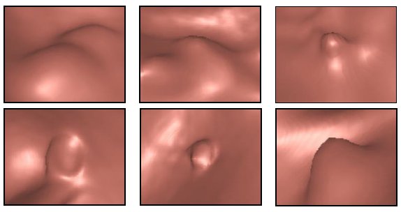
<body><![CDATA[<p align="center"> <font face="Verdana" size="2"> <a name="t3" href="/img/revistas/cleiej/v16n2/2a03t3.jpg"> Table 3: Results for the second test: Execution times for the sequential algorithm (CPU) and the parallel algorithm in CUDA (GPU) per dataset, test PC and kernel size. </a> </font> </p>       <p style='margin-top:0cm;margin-right:0cm;margin-bottom:5.95pt;margin-left: 0cm;text-align:justify;text-indent:0cm;mso-list:none;tab-stops:35.4pt'><b style='mso-bidi-font-weight:normal'><font face="Verdana"> <span lang=EN-US style='font-size:10pt; font-variant:normal;mso-ansi-language:EN-US'>5 Conclusion and Future Works</span></font><o:p></o:p></b></p>      <p style='margin-left:0cm;text-align:justify;text-indent:0cm;mso-list:none; tab-stops:35.4pt'><font face="Verdana"> <span lang=EN-US style='font-size:10.0pt;mso-bidi-font-size: 12.0pt;font-variant:normal;mso-ansi-language: EN-US'>In this work we have described the acceleration of an algorithm for the automatic detection of polyps, taking advantage of the parallelism provided by current graphics cards. Specifically, the detection was performed by curvature analysis, which requires the computation of the first and second order derivatives of the voxels in the colon wall. This computation was implemented in CUDA. The results show a reduction in execution time of up to 98% when comparing the CUDA version of the algorithm with a sequential version for CPU.<span style="mso-spacerun: yes">  </span>Several tests were also performed changing the amount of CUDA threads per block, but no significant change in the response time of the algorithm was observed between the different tests.</span></font><o:p></o:p></p>      <p style='margin-left:0cm;text-align:justify;text-indent:0cm'><![if !supportLists]> <span style='font-style:normal; font-variant:normal; font-weight:normal; font-size:10pt; font-family:Verdana; mso-bidi-font-size:12.0pt; mso-ansi-language:EN-US' lang="EN-US">&nbsp;&nbsp;&nbsp;&nbsp;&nbsp;&nbsp;&nbsp;&nbsp;&nbsp;&nbsp;&nbsp;&nbsp;&nbsp;&nbsp; </span><![endif]><font face="Verdana"> <span lang=EN-US style='font-size:10.0pt;mso-bidi-font-size: 12.0pt;font-variant:normal;mso-ansi-language: EN-US'>A new heuristic was implemented for removing polyp candidates which do not have the shape of a polyp. This heuristic consisted on analyzing the 2D shape of the candidate on a planar cut of the polyp, involving its perimeter and area. The amount of removed false positives with this heuristic is significant. Furthermore, the proposed that planar cut analysis could be easily integrated with other detection methods, such as the one developed by Kitasaka et al. <a href="#r7">(7)</a>.</span></font><o:p></o:p></p>      <p style='margin-left:0cm;text-align:justify;text-indent:0cm'><![if !supportLists]> <span style='font-style:normal; font-variant:normal; font-weight:normal; font-size:10pt; font-family:Verdana; mso-bidi-font-size:12.0pt; mso-ansi-language:EN-US' lang="EN-US">&nbsp;&nbsp;&nbsp;&nbsp;&nbsp;&nbsp;&nbsp;&nbsp;&nbsp;&nbsp;&nbsp;&nbsp;&nbsp;&nbsp; </span><![endif]><font face="Verdana"> <span lang=EN-US style='font-size:10.0pt;mso-bidi-font-size: 12.0pt;font-variant:normal;mso-ansi-language: EN-US'>The final polyp candidates obtained by our proposed algorithm are strong polyp candidates according to their shape. However, we could not compute the accuracy of our method because we do not have medical reports for all test datasets. </span></font> <o:p></o:p></p>      <p style='margin-left:0cm;text-align:justify;text-indent:0cm'><![if !supportLists]> <span style='font-style:normal; font-variant:normal; font-weight:normal; font-size:10pt; font-family:Verdana; mso-bidi-font-size:12.0pt; mso-ansi-language:EN-US' lang="EN-US">&nbsp;&nbsp;&nbsp;&nbsp;&nbsp;&nbsp;&nbsp;&nbsp;&nbsp;&nbsp;&nbsp;&nbsp;&nbsp;&nbsp; </span><![endif]><font face="Verdana"> <span lang=EN-US style='font-size:10.0pt;mso-bidi-font-size: 12.0pt;font-variant:normal;mso-ansi-language: EN-US'>As future work we propose performing more tests and analyzing the results with medical doctors for determining a concrete percentage of sensitivity and false positives rate. It would also be useful performing tests involving plain polyps, for determining whether our propose method can detect them or not. Additionally, the planar cut analysis could be used to segment the polyps out of the dataset. The idea would be moving the center of the cut in the direction of the normal forward and backwards, so as to obtain several cuts which comply with the conditions of the selective analysis and then select the voxels corresponding to the tissue region on every cut.</span></font><o:p></o:p></p>      <p><font face="Verdana" size="2"><span lang=EN-US>Acknowledgements</span></font></p>      <p style='text-align:justify'><font face="Verdana"><span lang=EN-US style='font-size:10.0pt;mso-bidi-font-size:12.0pt;mso-ansi-language:EN-US'>This work has been financed by the “Centro de Desarrollo Científico y Humanístico de la Universidad Central de Venezuela (CDCH-UCV)”, under project PG 03-00-6515-2006. The screenshots of the detected polyp candidates were captured using the CT Colonography module of Biotronics3D’s 3Dnet Suite (</span><span lang=EN-US style='mso-ansi-language:EN-US'><a href="http://www.3dnetsuite.com/"><span style='font-size:10.0pt;mso-bidi-font-size:12.0pt'>http://www.3dnetsuite.com/</span></a></span></font><span lang=EN-US style='font-size:10.0pt;mso-bidi-font-size:12.0pt;mso-ansi-language: EN-US'><font face="Verdana">).</font><o:p></o:p></span></p>      <p><span lang=ES-VE style='mso-ansi-language:ES-VE'> <font face="Verdana" size="2">References</font><o:p></o:p></span></p>      <!-- ref --><p style='margin-left:21.25pt;text-indent:-21.25pt;mso-pagination: widow-orphan;mso-list:l6 level1 lfo38'><![if !supportLists]><span style='mso-ansi-language:ES;mso-fareast-language:ES-VE'> <font face="Verdana" size="2"><a name="r1">(1)</a></font><span style='font-style:normal; font-variant:normal; font-weight:normal; font-size:10pt; font-family:Verdana'>&nbsp;&nbsp;&nbsp;&nbsp;&nbsp;&nbsp; </span></span> <![endif]><font face="Verdana" size="2"><i style='mso-bidi-font-style:normal'><span lang=ES-VE style='mso-ansi-language: ES-VE'>Anuario de Mortalidad 2008</span></i><span lang=ES-VE style='mso-ansi-language: ES-VE'>. Ministerio del Poder Popular para la Salud. República Bolivariana de Venezuela. </span><span lang=EN-US>May 2010. </span><span style='mso-ansi-language: ES'><a href="http://www.bvs.org.ve/anuario/anuario_2008.pdf">http://www.bvs.org.ve/anuario/anuario_2008.pdf</a>.    </span></font><span style='mso-ansi-language:ES;mso-fareast-language:ES-VE'><o:p></o:p></span></p>      <!-- ref --><p style='margin-left:21.25pt;text-indent:-21.25pt;mso-pagination: widow-orphan;mso-list:l6 level1 lfo38'><![if !supportLists]><span lang=EN-US style='mso-fareast-language:ES-VE'><font face="Verdana" size="2"><a name="r2">(2)</a></font><span style='font-style:normal; font-variant:normal; font-weight:normal; font-size:10pt; font-family:Verdana'>&nbsp;&nbsp;&nbsp;&nbsp;&nbsp;&nbsp; </span></span><![endif]><font face="Verdana" size="2"><span lang=EN-US>“</span><span lang=EN-US style='mso-fareast-language:ES-VE'>Cancer”, <i style='mso-bidi-font-style:normal'>Fact Sheet No. 297</i>, Media Centre, <span style='mso-bidi-font-style:italic'>World Health Organization</span>, Feb. 2012. </span><span lang=EN-US><a href="http://www.who.int/mediacentre/factsheets/fs297/en/"><span style='mso-fareast-language:ES-VE'>http://www.who.int/mediacentre/factsheets/fs297/en/</span></a></span></font><span lang=EN-US style='mso-fareast-language:ES-VE'><o:p></o:p></span><!-- ref --><p style='margin-left:21.25pt;text-indent:-21.25pt;mso-pagination: widow-orphan;mso-list:l6 level1 lfo38'><![if !supportLists]><span lang=EN-US style='mso-fareast-language:ES-VE'><font face="Verdana" size="2"><a name="r3">(3)</a></font><span style='font-style:normal; font-variant:normal; font-weight:normal; font-size:10pt; font-family:Verdana'>&nbsp;&nbsp;&nbsp;&nbsp;&nbsp;&nbsp; </span></span><![endif]><font face="Verdana" size="2"><span lang=EN-US>H. Yoshida and J. Nappi, “Three-dimensional computer-aided diagnosis scheme for detection of colonic polyps”,<i style='mso-bidi-font-style:normal'> IEEE Transactions on Medical Imaging</i>, vol. 20, no. 12, pp. 1261–1274. Dec. 2001.    </span></font><span lang=EN-US style='mso-fareast-language:ES-VE'><o:p></o:p></span></p>      <!-- ref --><p style='margin-left:21.25pt;text-indent:-21.25pt;mso-pagination: widow-orphan;mso-list:l6 level1 lfo38'><![if !supportLists]><span lang=EN-US style='mso-fareast-language:ES-VE'><font face="Verdana" size="2"><a name="r4">(4)</a></font><span style='font-style:normal; font-variant:normal; font-weight:normal; font-size:10pt; font-family:Verdana'>&nbsp;&nbsp;&nbsp;&nbsp;&nbsp;&nbsp; </span></span><![endif]><font face="Verdana" size="2"><span lang=EN-US>V.F. van Ravesteijn, L. Zhao, C.P. Botha, F.H. Post, F.M. Vos and L.J. van Vliet. “<span style='mso-bidi-font-style: italic'>Combining Mesh, Volume, and Streamline Representations for Polyp Detection in CT Colonography”, in<i> Proceedings of the 6<sup>th</sup> IEEE International Symposium on Biomedical Imaging: From Nano to Macro</i></span>, pp. 907-910. Jul. 2009.    </span></font><span lang=EN-US style='mso-fareast-language: ES-VE'><o:p></o:p></span></p>      <!-- ref --><p style='margin-left:21.25pt;text-indent:-21.25pt;mso-pagination: widow-orphan;mso-list:l6 level1 lfo38'><![if !supportLists]><span lang=EN-US> <font face="Verdana" size="2"><a name="r5">(5)</a></font><span style='font-style:normal; font-variant:normal; font-weight:normal; font-size:10pt; font-family:Verdana'>&nbsp;&nbsp;&nbsp;&nbsp;&nbsp;&nbsp; </span></span> <![endif]><font face="Verdana" size="2"><span lang=EN-US>A. Huang, J. Li, R. Summers, N. Petrick and A.K. Hara, “Improving polyp detection algorithms for CT Colonography: Pareto front approach”, <i style='mso-bidi-font-style:normal'>Pattern Recognition Letters</i>, vol. 31, no. 11, pp. 1461–1469. Aug. 2010.    </span></font></p>      <!-- ref --><p style='margin-left:21.25pt;text-indent:-21.25pt;mso-pagination: widow-orphan;mso-list:l6 level1 lfo38'><![if !supportLists]><span lang=EN-US style='mso-fareast-language:ES-VE'><font face="Verdana" size="2"><a name="r6">(6)</a></font><span style='font-style:normal; font-variant:normal; font-weight:normal; font-size:10pt; font-family:Verdana'>&nbsp;&nbsp;&nbsp;&nbsp;&nbsp;&nbsp; </span></span><![endif]><font face="Verdana" size="2"><span lang=EN-US>L. Zhao, C. Botha, J. Bescos, R. Truyen, F. Vos and F. Post, “Lines of curvature for polyp detection in virtual colonoscopy”, <i style='mso-bidi-font-style:normal'>IEEE Transactions on Visualization and Computer Graphics</i>, vol. 12, no. 5, pp. 885–892. Sep. 2006.    </span></font><span lang=EN-US style='mso-fareast-language:ES-VE'><o:p></o:p></span></p>      ]]></body>
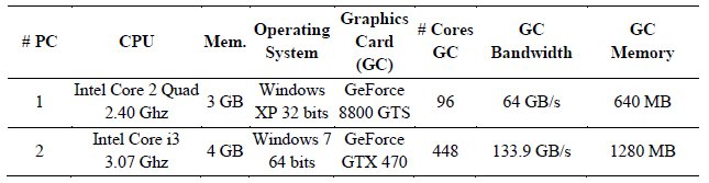
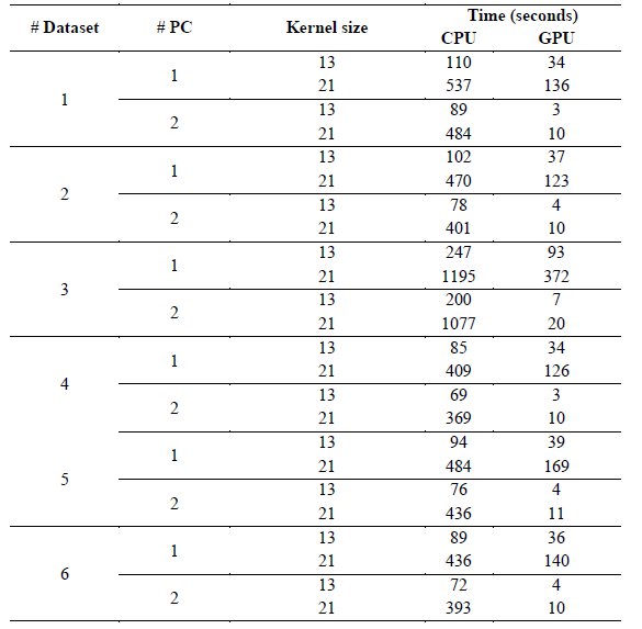
<body><![CDATA[<!-- ref --><p style='margin-left:21.25pt;text-indent:-21.25pt;mso-pagination: widow-orphan;mso-list:l6 level1 lfo38'><![if !supportLists]><span lang=EN-US> <font face="Verdana" size="2"><a name="r7">(7)</a></font><span style='font-style:normal; font-variant:normal; font-weight:normal; font-size:10pt; font-family:Verdana'>&nbsp;&nbsp;&nbsp;&nbsp;&nbsp;&nbsp; </span></span> <![endif]><font face="Verdana" size="2"><span lang=EN-US>T. Kitasaka, Y. Hayashi, T. Kimura, K. Mori, Y. Suenagac and J. Toriwaki, “Detection of colonic polyps from 3D abdominal CT images by surface fitting”, in <i style='mso-bidi-font-style:normal'>CARS 2005: Computer Assisted Radiology and Surgery</i>, vol. 1281, pp. 1151–1156. May 2005.    </span></font></p>      <!-- ref --><p style='margin-left:21.25pt;text-indent:-21.25pt;mso-pagination: widow-orphan;mso-list:l6 level1 lfo38'><![if !supportLists]><span lang=EN-US> <font face="Verdana" size="2"><a name="r8">(8)</a></font><span style='font-style:normal; font-variant:normal; font-weight:normal; font-size:10pt; font-family:Verdana'>&nbsp;&nbsp;&nbsp;&nbsp;&nbsp;&nbsp; </span></span> <![endif]><font face="Verdana" size="2"><span lang=EN-US>E. Konukoglu and B. Acar, “HDF: Heat diffusion fields for polyp detection in CT Colonography”, Signal Processing, vol. 87, no. 10, pp. 2407–2416. Oct. 2007.    </span></font></p>      <!-- ref --><p style='margin-left:21.25pt;text-indent:-21.25pt;mso-pagination: widow-orphan;mso-list:l6 level1 lfo38'><![if !supportLists]><span lang=EN-US style='mso-fareast-language:ES-VE'><font face="Verdana" size="2"><a name="r9">(9)</a></font><span style='font-style:normal; font-variant:normal; font-weight:normal; font-size:10pt; font-family:Verdana'>&nbsp;&nbsp;&nbsp;&nbsp;&nbsp;&nbsp; </span></span><![endif]><font face="Verdana" size="2"><span lang=EN-US>I. Bitter, B. Aslam, A. Huang and R. Summers, “Candidate determination for computer aided detection of colon polyps”, in <i style='mso-bidi-font-style:normal'>Medical Imaging 2005: Physiology, Function, and Structure from Medical Images</i>. A. Amini and A. Manduca (Eds.), pp. 804–809. Apr. 2005.    </span></font><span lang=EN-US style='mso-fareast-language: ES-VE'><o:p></o:p></span></p>      <!-- ref --><p style='margin-left:21.25pt;text-indent:-21.25pt;mso-pagination: widow-orphan;mso-list:l6 level1 lfo38'><![if !supportLists]><span lang=EN-US style='mso-fareast-language:ES-VE'><font face="Verdana" size="2"><a name="r10">(10)</a></font><span style='font-style:normal; font-variant:normal; font-weight:normal; font-size:10pt; font-family:Verdana'>&nbsp;&nbsp;&nbsp; </span></span><![endif]><font face="Verdana" size="2"><i style='mso-bidi-font-style:normal'><span lang=EN-US>CUDA Home</span></i><span lang=EN-US>. NVIDIA Corporation. 2011. <a href="http://www.nvidia.com/object/cuda_home_new.html">http://www.nvidia.com/object/cuda_home_new.html</a></span></font><span lang=EN-US style='mso-fareast-language:ES-VE'><o:p></o:p></span><!-- ref --><p style='margin-left:21.25pt;text-indent:-21.25pt;mso-pagination: widow-orphan;mso-list:l6 level1 lfo38'><![if !supportLists]><span lang=EN-US> <font face="Verdana" size="2"><a name="r11">(11)</a></font><span style='font-style:normal; font-variant:normal; font-weight:normal; font-size:10pt; font-family:Verdana'>&nbsp;&nbsp;&nbsp; </span></span> <![endif]><font face="Verdana" size="2"><span lang=EN-US>S. Gokturk and C. Tomasi, “A New 3-D Pattern Recognition Technique with Application to Computer Aided Colonoscopy”, in <i style='mso-bidi-font-style: normal'>Proceedings of the 2001 IEEE Computer Science Conference on Computer Vision and Pattern Recognition (CVPR)</i>, vol. 1, pp. 93-100. Dec. 2001.     </span> </font></p>      <!-- ref --><p style='margin-left:21.25pt;text-indent:-21.25pt;mso-pagination: widow-orphan;mso-list:l6 level1 lfo38'><![if !supportLists]><span lang=EN-US> <font face="Verdana" size="2"><a name="r12">(12)</a></font><span style='font-style:normal; font-variant:normal; font-weight:normal; font-size:10pt; font-family:Verdana'>&nbsp;&nbsp;&nbsp; </span></span> <![endif]><font face="Verdana" size="2"><span lang=EN-US>D. Paik, C. Beaulieu, G. Rubin, B. Acar, R. Jeffrey Jr., J. Yee, J. Dey and S. Napel. “Surface normal overlap: a Computer-Aided Detection Algorithm with application to Colonic Polyps and Lung Nodules in Helical CT”, <i style='mso-bidi-font-style:normal'>IEEE Transactions On Medical Imaging</i>, vol. 23, no. 6, pp. 661–675. Jun. 2004.    </span></font></p>      <!-- ref --><p style='margin-left:21.25pt;text-indent:-21.25pt;mso-pagination: widow-orphan;mso-list:l6 level1 lfo38'><![if !supportLists]><span lang=EN-US> <font face="Verdana" size="2"><a name="r13">(13)</a></font><span style='font-style:normal; font-variant:normal; font-weight:normal; font-size:10pt; font-family:Verdana'>&nbsp;&nbsp;&nbsp; </span></span> <![endif]><font face="Verdana" size="2"><span lang=EN-US>W. Lorensen and H. Cline, “Marching Cubes: A high resolution 3D surface construction algorithm”, <i style='mso-bidi-font-style:normal'>ACM</i> <i style='mso-bidi-font-style:normal'>SIGGRAPH</i> <i style='mso-bidi-font-style: normal'>Computer Graphics</i>, vol. 21, no. 4, pp. 163–169. Jul. 1987.    </span></font></p>      <!-- ref --><p style='margin-left:21.25pt;text-indent:-21.25pt;mso-pagination: widow-orphan;mso-list:l6 level1 lfo38'><![if !supportLists]><span lang=EN-US> <font face="Verdana" size="2"><a name="r14">(14)</a></font><span style='font-style:normal; font-variant:normal; font-weight:normal; font-size:10pt; font-family:Verdana'>&nbsp;&nbsp;&nbsp; </span></span> <![endif]><font face="Verdana" size="2"><span lang=EN-US>F. Qiu, Z. Fan, X. Yin, A. Kaufman and X.D. Gu, “Colon flattening with Discrete Ricci Flow”, in <i style='mso-bidi-font-style:normal'>Proceedings of the MICCAI 2008 Workshop: Computational and Visualization Challenges in the New Era of Virtual Colonoscopy,</i> pp. 97–102. Sep. 2008.    </span></font></p>      <!-- ref --><p style='margin-left:21.25pt;text-indent:-21.25pt;mso-pagination: widow-orphan;mso-list:l6 level1 lfo38'><![if !supportLists]><span lang=EN-US> <font face="Verdana" size="2"><a name="r15">(15)</a></font><span style='font-style:normal; font-variant:normal; font-weight:normal; font-size:10pt; font-family:Verdana'>&nbsp;&nbsp;&nbsp; </span></span> <![endif]><font face="Verdana" size="2"><span lang=EN-US>E. Coto and S. Grimm, “Improved data processing for virtual colonoscopy”, in <i style='mso-bidi-font-style:normal'>Proceedings of the IV Iberoamerican Symposium in Computer Graphics (SIACG 2009)</i>,<i style='mso-bidi-font-style:normal'> </i>O. Rodriguez et al. (Eds.), pp. 171–179. Jun. 2009.    </span></font></p>      <!-- ref --><p style='margin-left:21.25pt;text-indent:-21.25pt;mso-pagination: widow-orphan;mso-list:l6 level1 lfo38'><![if !supportLists]><span lang=EN-US> <font face="Verdana" size="2"><a name="r16">(16)</a></font><span style='font-style:normal; font-variant:normal; font-weight:normal; font-size:10pt; font-family:Verdana'>&nbsp;&nbsp;&nbsp; </span></span> <![endif]><font face="Verdana" size="2"><span lang=EN-US>O. Monga and S. Benayoun, “Using partial derivatives of 3D images to extract typical surface features”, in <i style='mso-bidi-font-style:normal'>Proceedings of the Third Annual Conference of AI, Simulation and Planning in High Autonomy Systems: Integrating Perception, Planning and Action</i>, pp. 225-236. Jul. 1992.    </span></font></p>      <!-- ref --><p style='margin-left:21.25pt;text-indent:-21.25pt;mso-pagination: widow-orphan;mso-list:l6 level1 lfo38'><![if !supportLists]><span lang=EN-US> <font face="Verdana" size="2"><a name="r17">(17)</a></font><span style='font-style:normal; font-variant:normal; font-weight:normal; font-size:10pt; font-family:Verdana'>&nbsp;&nbsp;&nbsp; </span></span> <![endif]><font face="Verdana" size="2"><span lang=EN-US>T. Möller, K. Mueller, Y. Kurzion, R. Machiraju and R. Yagel, “Design of accurate and smooth filters for function and derivative reconstruction”, in <i style='mso-bidi-font-style:normal'>Proceedings of the IEEE Symposium on Volume Visualization 1998</i>, pp. 143–151. Oct. 1998.     </span> </font></p>      <!-- ref --><p style='margin-left:21.25pt;text-indent:-21.25pt;mso-pagination: widow-orphan;mso-list:l6 level1 lfo38'><![if !supportLists]><span lang=EN-US> <font face="Verdana" size="2"><a name="r18">(18)</a></font><span style='font-style:normal; font-variant:normal; font-weight:normal; font-size:10pt; font-family:Verdana'>&nbsp;&nbsp;&nbsp; </span></span> <![endif]><font face="Verdana" size="2"><i style='mso-bidi-font-style:normal'><span lang=EN-US>VolVis.org</span></i><span lang=EN-US>. <a href="http://www.volvis.org/">http://www.volvis.org</a>.    </span></font></p>      <!-- ref --><p style='margin-left:21.25pt;text-indent:-21.25pt;mso-pagination: widow-orphan;mso-list:l6 level1 lfo38'><![if !supportLists]><span lang=EN-US> <font face="Verdana" size="2"><a name="r19">(19)</a></font><span style='font-style:normal; font-variant:normal; font-weight:normal; font-size:10pt; font-family:Verdana'>&nbsp;&nbsp;&nbsp; </span></span> <![endif]><font face="Verdana" size="2"><span lang=EN-US>M. Wan, F. Dachille, K. Kreeger, S. Lakare, M. Sato, A. Kaufman, M. Wax and Z. Liang, “Interactive electronic biopsy for 3D virtual colonoscopy,” in <i style='mso-bidi-font-style:normal'>Physiology and Function from Multidimensional Images</i>, ser. Proceedings of SPIE, C. Chen and A. Clough (Eds.), vol. 4321, pp. 483–488. May 2001.    </span></font></p>      <p style='margin-left:21.3pt;text-indent:-21.3pt;mso-pagination: widow-orphan'><span lang=EN-US><font face="Verdana" size="2"><![if !supportEmptyParas]>&nbsp;<![endif]></font><o:p></o:p></span></p>      <p style='margin-left:21.3pt;text-indent:-21.3pt;mso-pagination: widow-orphan'><span lang=EN-US><font face="Verdana" size="2"><![if !supportEmptyParas]>&nbsp;<![endif]></font><o:p></o:p></span></p>      <p><span lang=EN-US style='mso-ansi-language:EN-US'> <font face="Verdana" size="2"><![if !supportEmptyParas]>&nbsp;<![endif]></font><o:p></o:p></span></p>      <p style='text-align:justify'><span lang=EN-US style='mso-ansi-language:EN-US'><font face="Verdana" size="2"><![if !supportEmptyParas]>&nbsp;<![endif]></font><o:p></o:p></span></p>  </div>       ]]></body><back>
<ref-list>
<ref id="B1">
<label>1</label><nlm-citation citation-type="book">
<source><![CDATA[Anuario de Mortalidad 2008]]></source>
<year>May </year>
<month>20</month>
<day>10</day>
<publisher-name><![CDATA[Ministerio del Poder Popular para la Salud]]></publisher-name>
</nlm-citation>
</ref>
<ref id="B2">
<label>2</label><nlm-citation citation-type="book">
<source><![CDATA[Cancer]]></source>
<year>Feb.</year>
<month> 2</month>
<day>01</day>
<publisher-name><![CDATA[World Health Organization]]></publisher-name>
</nlm-citation>
</ref>
<ref id="B3">
<label>3</label><nlm-citation citation-type="journal">
<person-group person-group-type="author">
<name>
<surname><![CDATA[Yoshida]]></surname>
<given-names><![CDATA[H]]></given-names>
</name>
<name>
<surname><![CDATA[Napp]]></surname>
<given-names><![CDATA[J]]></given-names>
</name>
</person-group>
<article-title xml:lang="en"><![CDATA[“Three-dimensional computer-aided diagnosis scheme for detection of colonic polyps”]]></article-title>
<source><![CDATA[Transactions on Medical Imaging]]></source>
<year>Dec.</year>
<month> 2</month>
<day>00</day>
<volume>20</volume>
<numero>12</numero>
<issue>12</issue>
<page-range>1261-1274</page-range></nlm-citation>
</ref>
<ref id="B4">
<label>4</label><nlm-citation citation-type="confpro">
<person-group person-group-type="author">
<name>
<surname><![CDATA[van Ravesteijn]]></surname>
<given-names><![CDATA[V.F]]></given-names>
</name>
<name>
<surname><![CDATA[Zhao]]></surname>
<given-names><![CDATA[L]]></given-names>
</name>
<name>
<surname><![CDATA[Botha]]></surname>
<given-names><![CDATA[C.P]]></given-names>
</name>
<name>
<surname><![CDATA[Post]]></surname>
<given-names><![CDATA[F.H]]></given-names>
</name>
<name>
<surname><![CDATA[Vos]]></surname>
<given-names><![CDATA[F.M]]></given-names>
</name>
<name>
<surname><![CDATA[van Vliet]]></surname>
<given-names><![CDATA[L.J]]></given-names>
</name>
</person-group>
<source><![CDATA[“Combining Mesh, Volume, and Streamline Representations for Polyp Detection in CT Colonography”]]></source>
<year>Jul.</year>
<month> 2</month>
<day>00</day>
<conf-name><![CDATA[ 6th IEEE International Symposium on Biomedical Imaging]]></conf-name>
<conf-loc> </conf-loc>
<page-range>907-910</page-range><publisher-name><![CDATA[From Nano to Macro]]></publisher-name>
</nlm-citation>
</ref>
<ref id="B5">
<label>5</label><nlm-citation citation-type="journal">
<person-group person-group-type="author">
<name>
<surname><![CDATA[Huang]]></surname>
<given-names><![CDATA[A]]></given-names>
</name>
<name>
<surname><![CDATA[L]]></surname>
<given-names><![CDATA[J]]></given-names>
</name>
<name>
<surname><![CDATA[Summers]]></surname>
<given-names><![CDATA[R]]></given-names>
</name>
<name>
<surname><![CDATA[Petrick]]></surname>
<given-names><![CDATA[N]]></given-names>
</name>
<name>
<surname><![CDATA[Hara]]></surname>
<given-names><![CDATA[A.K]]></given-names>
</name>
</person-group>
<article-title xml:lang="en"><![CDATA[“Improving polyp detection algorithms for CT Colonography: Pareto front approach]]></article-title>
<source><![CDATA[Pattern Recognition Letters]]></source>
<year>Aug.</year>
<month> 2</month>
<day>01</day>
<volume>31</volume>
<numero>11</numero>
<issue>11</issue>
<page-range>1461-1469</page-range></nlm-citation>
</ref>
<ref id="B6">
<label>6</label><nlm-citation citation-type="journal">
<person-group person-group-type="author">
<name>
<surname><![CDATA[Zhao]]></surname>
<given-names><![CDATA[L]]></given-names>
</name>
<name>
<surname><![CDATA[Botha]]></surname>
<given-names><![CDATA[C]]></given-names>
</name>
<name>
<surname><![CDATA[Bescos]]></surname>
<given-names><![CDATA[J]]></given-names>
</name>
<name>
<surname><![CDATA[Truyen]]></surname>
<given-names><![CDATA[R]]></given-names>
</name>
<name>
<surname><![CDATA[Vos]]></surname>
<given-names><![CDATA[F]]></given-names>
</name>
<name>
<surname><![CDATA[Post]]></surname>
<given-names><![CDATA[F]]></given-names>
</name>
</person-group>
<article-title xml:lang="en"><![CDATA[“Lines of curvature for polyp detection in virtual colonoscopy”]]></article-title>
<source><![CDATA[IEEE Transactions on Visualization and Computer Graphics]]></source>
<year>Sep.</year>
<month> 2</month>
<day>00</day>
<volume>12</volume>
<numero>5</numero>
<issue>5</issue>
<page-range>885-892</page-range></nlm-citation>
</ref>
<ref id="B7">
<label>7</label><nlm-citation citation-type="">
<person-group person-group-type="author">
<name>
<surname><![CDATA[Kitasaka]]></surname>
<given-names><![CDATA[T]]></given-names>
</name>
<name>
<surname><![CDATA[Hayashi]]></surname>
<given-names><![CDATA[Y]]></given-names>
</name>
<name>
<surname><![CDATA[Kimura]]></surname>
<given-names><![CDATA[T]]></given-names>
</name>
<name>
<surname><![CDATA[Mori]]></surname>
<given-names><![CDATA[K]]></given-names>
</name>
<name>
<surname><![CDATA[Suenagac]]></surname>
<given-names><![CDATA[Y]]></given-names>
</name>
<name>
<surname><![CDATA[Toriwaki]]></surname>
<given-names><![CDATA[J]]></given-names>
</name>
</person-group>
<source><![CDATA[“Detection of colonic polyps from 3D abdominal CT images by surface fitting”: in CARS 2005: Computer Assisted Radiology and Surgery]]></source>
<year>May </year>
<month>20</month>
<day>05</day>
<volume>1281</volume>
<page-range>1151-1156</page-range></nlm-citation>
</ref>
<ref id="B8">
<label>8</label><nlm-citation citation-type="journal">
<person-group person-group-type="author">
<name>
<surname><![CDATA[Konukoglu]]></surname>
<given-names><![CDATA[E]]></given-names>
</name>
<name>
<surname><![CDATA[Acar]]></surname>
<given-names><![CDATA[B]]></given-names>
</name>
</person-group>
<article-title xml:lang="en"><![CDATA[“HDF: Heat diffusion fields for polyp detection in CT Colonography”]]></article-title>
<source><![CDATA[Signal Processing]]></source>
<year>Oct.</year>
<month> 2</month>
<day>00</day>
<volume>. 87</volume>
<numero>10</numero>
<issue>10</issue>
<page-range>2407-2416</page-range></nlm-citation>
</ref>
<ref id="B9">
<label>9</label><nlm-citation citation-type="journal">
<person-group person-group-type="author">
<name>
<surname><![CDATA[Bitter]]></surname>
<given-names><![CDATA[I]]></given-names>
</name>
<name>
<surname><![CDATA[Aslam]]></surname>
<given-names><![CDATA[B]]></given-names>
</name>
<name>
<surname><![CDATA[Huang]]></surname>
<given-names><![CDATA[A]]></given-names>
</name>
<name>
<surname><![CDATA[Summers]]></surname>
<given-names><![CDATA[R]]></given-names>
</name>
</person-group>
<article-title xml:lang="en"><![CDATA[Candidate determination for computer aided detection of colon polyps]]></article-title>
<source><![CDATA[Medical Imaging 2005]]></source>
<year>Apr.</year>
<month> 2</month>
<day>00</day>
<page-range>804-809</page-range><publisher-name><![CDATA[A. Amini and A. Manduca]]></publisher-name>
</nlm-citation>
</ref>
<ref id="B10">
<label>10</label><nlm-citation citation-type="">
<source><![CDATA[CUDA Home. NVIDIA Corporation]]></source>
<year>2011</year>
</nlm-citation>
</ref>
<ref id="B11">
<label>11</label><nlm-citation citation-type="">
<person-group person-group-type="author">
<name>
<surname><![CDATA[Gokturk]]></surname>
<given-names><![CDATA[S]]></given-names>
</name>
<name>
<surname><![CDATA[Tomasi]]></surname>
<given-names><![CDATA[C]]></given-names>
</name>
</person-group>
<article-title xml:lang="en"><![CDATA[A New 3-D Pattern Recognition Technique with Application to Computer Aided Colonoscopy]]></article-title>
<source><![CDATA[]]></source>
<year></year>
</nlm-citation>
</ref>
<ref id="B12">
<label>12</label><nlm-citation citation-type="journal">
<person-group person-group-type="author">
<name>
<surname><![CDATA[Paik]]></surname>
<given-names><![CDATA[D]]></given-names>
</name>
<name>
<surname><![CDATA[Beaulieu]]></surname>
<given-names><![CDATA[C]]></given-names>
</name>
<name>
<surname><![CDATA[Rubin]]></surname>
<given-names><![CDATA[G]]></given-names>
</name>
<name>
<surname><![CDATA[Acar]]></surname>
<given-names><![CDATA[B]]></given-names>
</name>
<name>
<surname><![CDATA[Jeffrey]]></surname>
<given-names><![CDATA[R]]></given-names>
</name>
<name>
<surname><![CDATA[Yee]]></surname>
<given-names><![CDATA[J]]></given-names>
</name>
<name>
<surname><![CDATA[Dey]]></surname>
<given-names><![CDATA[J]]></given-names>
</name>
<name>
<surname><![CDATA[Napel]]></surname>
<given-names><![CDATA[S]]></given-names>
</name>
</person-group>
<article-title xml:lang="en"><![CDATA[Surface normal overlap: a Computer-Aided Detection Algorithm with application to Colonic Polyps and Lung Nodules in Helical CT]]></article-title>
<source><![CDATA[IEEE Transactions On Medical Imaging]]></source>
<year>Jun.</year>
<month> 2</month>
<day>00</day>
<volume>23</volume>
<numero>6</numero>
<issue>6</issue>
<page-range>661-675</page-range></nlm-citation>
</ref>
<ref id="B13">
<label>13</label><nlm-citation citation-type="journal">
<person-group person-group-type="author">
<name>
<surname><![CDATA[Lorensen]]></surname>
<given-names><![CDATA[W]]></given-names>
</name>
<name>
<surname><![CDATA[Cline]]></surname>
<given-names><![CDATA[H]]></given-names>
</name>
</person-group>
<article-title xml:lang="en"><![CDATA[Marching Cubes: A high resolution 3D surface construction algorithm]]></article-title>
<source><![CDATA[ACM SIGGRAPH Computer Graphics]]></source>
<year>Jul.</year>
<month> 1</month>
<day>98</day>
<volume>21</volume>
<numero>4</numero>
<issue>4</issue>
<page-range>163-169</page-range></nlm-citation>
</ref>
<ref id="B14">
<label>14</label><nlm-citation citation-type="">
<person-group person-group-type="author">
<name>
<surname><![CDATA[Qiu]]></surname>
<given-names><![CDATA[F]]></given-names>
</name>
<name>
<surname><![CDATA[Fan]]></surname>
<given-names><![CDATA[Z]]></given-names>
</name>
<name>
<surname><![CDATA[Yin]]></surname>
<given-names><![CDATA[X]]></given-names>
</name>
<name>
<surname><![CDATA[Kaufman]]></surname>
<given-names><![CDATA[A]]></given-names>
</name>
<name>
<surname><![CDATA[Gu]]></surname>
<given-names><![CDATA[X.D]]></given-names>
</name>
</person-group>
<article-title xml:lang="en"><![CDATA[Colon flattening with Discrete Ricci Flow]]></article-title>
<source><![CDATA[]]></source>
<year></year>
</nlm-citation>
</ref>
<ref id="B15">
<label>15</label><nlm-citation citation-type="">
<person-group person-group-type="author">
<name>
<surname><![CDATA[Coto]]></surname>
<given-names><![CDATA[E]]></given-names>
</name>
<name>
<surname><![CDATA[Grimm]]></surname>
<given-names><![CDATA[S]]></given-names>
</name>
</person-group>
<article-title xml:lang="en"><![CDATA[Improved data processing for virtual colonoscopy]]></article-title>
<source><![CDATA[]]></source>
<year></year>
</nlm-citation>
</ref>
<ref id="B16">
<label>16</label><nlm-citation citation-type="">
<person-group person-group-type="author">
<name>
<surname><![CDATA[Monga]]></surname>
<given-names><![CDATA[O]]></given-names>
</name>
<name>
<surname><![CDATA[Benayoun]]></surname>
<given-names><![CDATA[S]]></given-names>
</name>
</person-group>
<article-title xml:lang="en"><![CDATA[Using partial derivatives of 3D images to extract typical surface features]]></article-title>
<source><![CDATA[]]></source>
<year></year>
</nlm-citation>
</ref>
<ref id="B17">
<label>17</label><nlm-citation citation-type="">
<person-group person-group-type="author">
<name>
<surname><![CDATA[Möller]]></surname>
<given-names><![CDATA[T]]></given-names>
</name>
<name>
<surname><![CDATA[Mueller]]></surname>
<given-names><![CDATA[K]]></given-names>
</name>
<name>
<surname><![CDATA[Kurzion]]></surname>
<given-names><![CDATA[Y]]></given-names>
</name>
<name>
<surname><![CDATA[Machiraju]]></surname>
<given-names><![CDATA[R]]></given-names>
</name>
<name>
<surname><![CDATA[Yagel]]></surname>
<given-names><![CDATA[R]]></given-names>
</name>
</person-group>
<article-title xml:lang="en"><![CDATA[Design of accurate and smooth filters for function and derivative reconstruction]]></article-title>
<source><![CDATA[]]></source>
<year></year>
</nlm-citation>
</ref>
<ref id="B18">
<label>18</label><nlm-citation citation-type="">
<source><![CDATA[VolVis.org]]></source>
<year></year>
</nlm-citation>
</ref>
<ref id="B19">
<label>19</label><nlm-citation citation-type="book">
<person-group person-group-type="author">
<name>
<surname><![CDATA[Wan]]></surname>
<given-names><![CDATA[M]]></given-names>
</name>
<name>
<surname><![CDATA[Dachille]]></surname>
<given-names><![CDATA[F]]></given-names>
</name>
<name>
<surname><![CDATA[Kreeger]]></surname>
<given-names><![CDATA[K]]></given-names>
</name>
<name>
<surname><![CDATA[Lakare]]></surname>
<given-names><![CDATA[S]]></given-names>
</name>
<name>
<surname><![CDATA[Sato]]></surname>
<given-names><![CDATA[M]]></given-names>
</name>
<name>
<surname><![CDATA[Kaufman]]></surname>
<given-names><![CDATA[A]]></given-names>
</name>
<name>
<surname><![CDATA[Wax]]></surname>
<given-names><![CDATA[M]]></given-names>
</name>
<name>
<surname><![CDATA[Liang]]></surname>
<given-names><![CDATA[Z]]></given-names>
</name>
</person-group>
<source><![CDATA[Physiology and Function from Multidimensional Images]]></source>
<year>May </year>
<month>20</month>
<day>01</day>
<volume>4321</volume>
<page-range>483-488</page-range><publisher-name><![CDATA[C. Chen and A. Clough]]></publisher-name>
</nlm-citation>
</ref>
</ref-list>
</back>
</article>