<?xml version="1.0" encoding="ISO-8859-1"?><article xmlns:mml="http://www.w3.org/1998/Math/MathML" xmlns:xlink="http://www.w3.org/1999/xlink" xmlns:xsi="http://www.w3.org/2001/XMLSchema-instance">
<front>
<journal-meta>
<journal-id>0717-5000</journal-id>
<journal-title><![CDATA[CLEI Electronic Journal]]></journal-title>
<abbrev-journal-title><![CDATA[CLEIej]]></abbrev-journal-title>
<issn>0717-5000</issn>
<publisher>
<publisher-name><![CDATA[Centro Latinoamericano de Estudios en Informática]]></publisher-name>
</publisher>
</journal-meta>
<article-meta>
<article-id>S0717-50002012000300002</article-id>
<title-group>
<article-title xml:lang="en"><![CDATA[Parallel Adaptive Simulation of Coupled Incompressible Viscous Flow and Advective-Diffusive Transport Using Stabilized FEM Formulation]]></article-title>
</title-group>
<contrib-group>
<contrib contrib-type="author">
<name>
<surname><![CDATA[L. Rossa]]></surname>
<given-names><![CDATA[André]]></given-names>
</name>
<xref ref-type="aff" rid="A01"/>
</contrib>
<contrib contrib-type="author">
<name>
<surname><![CDATA[L.G.A. Coutinho]]></surname>
<given-names><![CDATA[Alvaro]]></given-names>
</name>
<xref ref-type="aff" rid="A02"/>
</contrib>
</contrib-group>
<aff id="A01">
<institution><![CDATA[,Engineering Simulation and Scientific Software  ]]></institution>
<addr-line><![CDATA[Rio de Janeiro ]]></addr-line>
<country>Brazil</country>
</aff>
<aff id="A02">
<institution><![CDATA[,High-Performance Computing Center  ]]></institution>
<addr-line><![CDATA[Rio de Janeiro ]]></addr-line>
<country>Brazil</country>
</aff>
<pub-date pub-type="pub">
<day>00</day>
<month>12</month>
<year>2012</year>
</pub-date>
<pub-date pub-type="epub">
<day>00</day>
<month>12</month>
<year>2012</year>
</pub-date>
<volume>15</volume>
<numero>3</numero>
<fpage>1</fpage>
<lpage>1</lpage>
<copyright-statement/>
<copyright-year/>
<self-uri xlink:href="http://www.scielo.edu.uy/scielo.php?script=sci_arttext&amp;pid=S0717-50002012000300002&amp;lng=en&amp;nrm=iso"></self-uri><self-uri xlink:href="http://www.scielo.edu.uy/scielo.php?script=sci_abstract&amp;pid=S0717-50002012000300002&amp;lng=en&amp;nrm=iso"></self-uri><self-uri xlink:href="http://www.scielo.edu.uy/scielo.php?script=sci_pdf&amp;pid=S0717-50002012000300002&amp;lng=en&amp;nrm=iso"></self-uri><abstract abstract-type="short" xml:lang="en"><p><![CDATA[Abstract In this work we study coupled incompressible viscous flow and advective-diffusive transport of a scalar. Both the Navier-Stokes and transport equations are solved using an Eulerian approach. The SUPG/PSPG stabilized finite element formulation is applied for the governing equations. The implementation is held using the libMEsh finite element library which provides support for parallel adaptive mesh refinement and coarsening. The Rayleigh-Bénard natural convection and the planar lock-exchange density current problems are solved to assess the adaptive parallel performance of the numerical solution.]]></p></abstract>
</article-meta>
</front><body><![CDATA[ <div class="maketitle">    <b><font face="Verdana" size="4">Parallel Adaptive Simulation of Coupled Incompressible Viscous Flow and Advective-Diffusive Transport Using Stabilized FEM Formulation</font></b>    <div class="author">    <font face="Verdana" size="2"> <span class="cmbx-12">Andr&eacute; L. Rossa</span>     <br>                    <span class="cmr-12">Engineering Simulation and Scientific Software,</span>     <br>                           <span class="cmr-12">Rio de Janeiro, Brazil, 20210-031,</span>     <br>                  <span class="cmti-12"><a href="mailto:andre.rossa@esss.com.br">andre.rossa@esss.com.br</a> </span><br class="and">     <span class="cmbx-12">Alvaro L.G.A. Coutinho</span>     <br>     <span class="cmr-12">High-Performance Computing Center, Department of Civil Engineering, UFRJ</span>     <br>                           <span class="cmr-12">Rio de Janeiro, Brazil, 21941-972</span>     <br>                                 <span class="cmti-12"><a href="mailto:alvaro@nacad.ufrj.br">alvaro@nacad.ufrj.br</a> </span>   </font></div>     <font face="Verdana" size="2">         <br>      </font>          <div class="date"></div>         </div>              ]]></body>
<body><![CDATA[<div class="abstract">     <div class="center"> <font face="Verdana" size="2">     <br>    </font>        <p> </p>         <div class="minipage">     <div class="center"> <font face="Verdana" size="2">     <br>    </font>        <p> </p>         <p><font face="Verdana" size="2"><span class="cmbx-10">Abstract</span></font></p>     </div>      <font face="Verdana" size="2">          <br>    </font>        ]]></body>
<body><![CDATA[<p><font face="Verdana" size="2">In this work we study coupled incompressible viscous flow and advective-diffusive transport of a scalar. Both the Navier-Stokes and transport equations are solved using an Eulerian approach. The SUPG/PSPG stabilized finite element formulation is applied for the governing equations. The implementation is held using the libMEsh finite element library which provides support for parallel adaptive mesh refinement and coarsening. The Rayleigh-B&eacute;nard natural convection and the planar lock-exchange density current problems are solved to assess the adaptive parallel performance of the numerical solution. <br class="newline">          <br>   </font>   </p>         <p><font face="Verdana" size="2"><span class="cmbx-10">Portuguese abstract </span><br class="newline">     Nesse trabalho n&oacute;s estudamos o escoamento incompress&iacute;vel de fluidos viscosos e o transporte advectivo-difusivo de um escalar. As equa&ccedil;&otilde;es de Navier-Stokes e do transporte s&atilde;o resolvidas usando um esquema Euleriano. A formula&ccedil;&atilde;o estabilizada SUPG/PSPG do m&eacute;todo dos elementos finitos &eacute; aplicada &agrave;s equa&ccedil;&otilde;es governantes. A implementa&ccedil;&atilde;o &eacute; realizada utilizando a biblioteca de elementos finitos libMesh que fornece suporte para refinamento/desrefinamento adaptativo de malhas em paralelo. Os problemas de convec&ccedil;&atilde;o natural de Rayleigh-B&eacute;nard e de corrente gravitacional em configura&ccedil;&atilde;o lock-exchange plana s&atilde;o resolvidos para avaliar o desempenho da solu&ccedil;&atilde;o num&eacute;rica paralela e adaptativa. </font> </p>     </div>     </div>      </div>      <font face="Verdana" size="2">          <br>    </font>        <p><font face="Verdana" size="2"><span class="cmbx-10">Keywords: </span>Stabilized FEM formulation, incompressible flows, adaptive meshes, parallel computing. <br class="newline">          <br>   </font>   </p>         <p> <font face="Verdana" size="2">Formula&ccedil;&atilde;o estabilizada do MEF, escoamentos incompress&iacute;veis, malhas adapatativas, computa&ccedil;&atilde;o paralela<br class="newline">          <br>   </font>   </p>         <p>   <font face="Verdana" size="2">Received: 2012-06-10 Revised 2012-10-01 Accepted 2012-10-04 </font>    </p>         <p><font face="Verdana" size="2"><span class="titlemark">1   </span> <a id="x1-10001"></a>Introduction</font></p>      <font face="Verdana" size="2">          ]]></body>
<body><![CDATA[<br>    </font>        <p><font face="Verdana" size="2">The numerical simulation of current engineering problems would not be feasible without the advent of parallel computing. Even with the development of techniques for mesh adaptation, the fastest available processors are not able to solve, within a practical period of time, problems that have large amounts of degrees of freedom. High-performance computing (HPC) have enabled the solution of problems with a large number of unknowns and high complexity (often involving multiple scales and multiple physics) by clusters of computers installed in universities as well in industry research centers.&nbsp;</font></p>         <p>   <font face="Verdana" size="2">To make HPC be efficiently used, a set of algorithms and computational methods have been developed over the last decade that made possible high fidelity solutions of complex problems. Processors with multiple cores with shared memory, clusters of personal computers in which each processor has its own memory (distributed memory) and more recently, the hybrid memory architectures are present on the daily work of engineers and researchers.&nbsp;</font></p>         <p>   <font face="Verdana" size="2">Although improving processing capacity, parallel computation have added complexity to computer codes programing. According to <span class="cite">(<a name="1."></a><a href="#1..">1</a>)</span> scaling performance is particularly problematic because the vision of seamless scalability cannot be achieved without having the applications scale automatically as the number of processors increases. However, for this to happen, the applications have to be programmed to exploit parallelism efficiently. Therefore, parallel computing resources should be used rationally in order to obtain compatible performances.&nbsp;</font></p>         <p>   <font face="Verdana" size="2">Good simulation practice suggests that the applications and algorithms employed in HPC should be optimized for this purpose. Currently there are available (mostly freely distributed) several programs to perform different tasks inherent to parallel computing. The domain partitioning and load balancing, information exchange between processors, algebraic operations and linear preconditioned systems solving are some of the necessary operations and have specific computational libraries that can be incorporated into the implementation of a numerical simulator.&nbsp;</font></p>         <p>   <font face="Verdana" size="2">In order to keep the focus on the issues related to the numerical problem, we use the <span class="obeylines-h"><span class="verb"><span class="cmtt-10">libMesh</span></span></span> framework, which is a C++ library for parallel adaptive mesh refinement/coarsening numerical multiphysics simulations based on the finite element method <span class="cite">(<a name="2."></a><a href="#2..">2</a>)</span>. The library has been developed since 2002 by a group of researchers from CFDLab, Department of Aerospace Engineering and Engineering Mechanics, University of Texas at Austin, and is available as open source software (<a href="http://libmesh.sourceforge.net/" class="url"><span class="cmtt-10">http://libmesh.sourceforge.net/</span></a>).&nbsp;</font></p>         <p>   <font face="Verdana" size="2">In this work we implement stabilized finite element formulations for the Navier-Stokes and advective-diffusive transport in <span class="obeylines-h"><span class="verb"><span class="cmtt-10">libMesh</span></span></span>. Parallel adaptive simulations of coupled problems confirm the mesh size reduction potential and the ability to capture the solution small scales as well the development of the interface between the fluids in evolution problems.&nbsp;</font></p>         <p>   <font face="Verdana" size="2">The remainder of this work is organized as follows. In the next section the dimensionless governing equations for the coupled viscous flow and transport is presented together with correspondent stabilized SUPG/PSPG finite element method (FEM) formulation. Details of the adaptive mesh refinement/coarsening (AMR/C) in the context of the <span class="obeylines-h"><span class="verb"><span class="cmtt-10">libMesh</span></span></span> library as well some aspects of the parallel solution of precondiotioned linear systems are presented in Section&nbsp;<a href="#x1-60003">3</a>. Section&nbsp;<a href="#x1-100004">4</a> presents the results of the parallel adaptive simulation of the Rayleigh-B&eacute;nard natural convection and a density current in a planar lock-exchange configuration. The paper ends with the main conclusions.&nbsp;</font></p>         <p>    </p>         <p><font face="Verdana" size="2"><span class="titlemark">2   </span> <a id="x1-20002"></a>Mathematical Formulation</font></p>      <font face="Verdana" size="2">          ]]></body>
<body><![CDATA[<br>    </font>        <p>    </p>         <p><font face="Verdana" size="2"><span class="titlemark">2.1   </span> <a id="x1-30002.1"></a>Governing Equations</font></p>      <font face="Verdana" size="2">          <br>    </font>        <p><font face="Verdana" size="2">Assuming an unsteady incompressible viscous flow and the Bousinessq approximation, the dimensionless Navier-Stokes, continuity and scalar transport equations (details on how the physical quantities may be normalized in order to arrive at dimensionless equations can be found at <span class="cite">(<a name="3."></a><a href="#3..">3</a>)</span>) can be written in a non conservative form following a Eulerian description as </font>    </p>     <table class="equation">       <tbody>         <tr>           <td><font face="Verdana" size="2"><a id="x1-3001r1"></a>                                        </font>                                        <center class="math-display">       <font face="Verdana" size="2">       <img src="/img/revistas/cleiej/v15n3/3a020x.png" alt="&part;u-        -1-  2        -Gr-  &part;t + u&nabla;u - Re &nabla; u+ &nabla;p = Re2 &#981;e   in  &Omega; &times;(0,t]," class="math-display"></font></center>           </td>           <td class="equation-label"><font face="Verdana" size="2">(<a href="#x1.">1</a>)</font></td>         </tr>                   </tbody> </table>      <font face="Verdana" size="2">          <br>    </font>        <p>    </p>     <table class="equation">       <tbody>         <tr>           <td><font face="Verdana" size="2"><a id="x1-3002r2"></a>                                       </font>                                       <center class="math-display">       <font face="Verdana" size="2">       <img src="/img/revistas/cleiej/v15n3/3a021x.png" alt="&nabla; &sdot;u = 0  in &Omega; &times; (0,t]," class="math-display"></font></center>           </td>           <td class="equation-label"><font face="Verdana" size="2">(2)</font></td>         </tr>                   </tbody> </table>      <font face="Verdana" size="2">          <br>    </font>        <p>    </p>     <table class="equation">       <tbody>         <tr>           <td><font face="Verdana" size="2"><a id="x1-3003r3"></a>                                       </font>                                       <center class="math-display">       <font face="Verdana" size="2">       <img src="/img/revistas/cleiej/v15n3/3a022x.png" alt="&part;&#981;-+ u&sdot;&nabla; &#981;- -1&nabla;2 &#981; = 0  in &Omega; &times; (0,t]. &part;t          D" class="math-display"></font></center>           </td>           <td class="equation-label"><font face="Verdana" size="2">(3)</font></td>         </tr>                   </tbody> </table>      <font face="Verdana" size="2">          <br>    </font>        ]]></body>
<body><![CDATA[<p> <font face="Verdana" size="2">defined in the simulation domain <img src="/img/revistas/cleiej/v15n3/3a023x.png" alt="&Omega;  " class="math"> with a smooth boundary <img src="/img/revistas/cleiej/v15n3/3a024x.png" alt="&Gamma;  " class="math">. The time is <img src="/img/revistas/cleiej/v15n3/3a025x.png" alt="t  " class="math">, <img src="/img/revistas/cleiej/v15n3/3a026x.png" alt="u = (u,v,w)T  " class="math"> is the velocity field, <img src="/img/revistas/cleiej/v15n3/3a027x.png" alt="p  " class="math"> is the pressure and <img src="/img/revistas/cleiej/v15n3/3a028x.png" alt="&#981;  " class="math"> the scalar being transported and <img src="/img/revistas/cleiej/v15n3/3a029x.png" alt="e  " class="math"> is an unit vector aligned with the gravity.&nbsp;</font></p>         <p>   <font face="Verdana" size="2">In (<a href="#x1-3001r1">1</a>) <img src="/img/revistas/cleiej/v15n3/3a0210x.png" alt="Re  " class="math"> and <img src="/img/revistas/cleiej/v15n3/3a0211x.png" alt="Gr  " class="math"> are the Reynolds and Grashof numbers. The inverse of the parameter <img src="/img/revistas/cleiej/v15n3/3a0212x.png" alt="D  " class="math"> in equation (<a href="#x1-3003r3">3</a>) represents a dimensionless diffusive constant depending on the nature of the scalar being transported (e.g., the Peclet number for the temperature transport).&nbsp;</font></p>         <p>   <font face="Verdana" size="2">The essential and natural boundaries conditions (BCs) are: </font>    </p>     <table class="equation">       <tbody>         <tr>           <td><font face="Verdana" size="2"><a id="x1-3004r4"></a>                                       </font>                                       <center class="math-display">       <font face="Verdana" size="2">       <img src="/img/revistas/cleiej/v15n3/3a0213x.png" alt="  (                    u] = g   on &Gamma; g,     1--(         T) n&sdot;  Re  &nabla;u + (&nabla;u )   - pI = h   on &Gamma; &sigma;,                        &#981; = &#981;-  on &Gamma; ,                  (     )           &#981;              - n &sdot;-1&nabla; &#981;  = q    on &Gamma; q                   D" class="math-display"></font></center>           </td>           <td class="equation-label"><font face="Verdana" size="2">(4)</font></td>         </tr>                   </tbody> </table>      <font face="Verdana" size="2">          <br>   </font>       <p> <font face="Verdana" size="2">where <img src="/img/revistas/cleiej/v15n3/3a0214x.png" alt="g  " class="math"> and <img src="/img/revistas/cleiej/v15n3/3a0215x.png" alt="-- &#981;  " class="math"> are functions with prescribed values for the velocity vector and scalar defined on the regions <img src="/img/revistas/cleiej/v15n3/3a0216x.png" alt="&Gamma; g  " class="math"> and <img src="/img/revistas/cleiej/v15n3/3a0217x.png" alt="&Gamma; &#981;  " class="math"> of the boundary where the essential BCs are imposed. Furthermore <img src="/img/revistas/cleiej/v15n3/3a0218x.png" alt="h  " class="math"> and <img src="/img/revistas/cleiej/v15n3/3a0219x.png" alt="q  " class="math"> represent the natural BCs acting on the regions <img src="/img/revistas/cleiej/v15n3/3a0220x.png" alt="&Gamma; &sigma; " class="math"> and <img src="/img/revistas/cleiej/v15n3/3a0221x.png" alt="&Gamma; q  " class="math">. Generally <img src="/img/revistas/cleiej/v15n3/3a0222x.png" alt="&Gamma; i &sub; &Gamma;  " class="math">. <img src="/img/revistas/cleiej/v15n3/3a0223x.png" alt="n  " class="math"> is the unit outward normal vector on the boundary and <img src="/img/revistas/cleiej/v15n3/3a0224x.png" alt="I  " class="math"> is the <img src="/img/revistas/cleiej/v15n3/3a0225x.png" alt="/img/revistas/cleiej/v15n3/3 &times; 3  " class="math"> identity matrix.&nbsp;</font></p>         <p>   <font face="Verdana" size="2">The initial conditions are: </font>    </p>     <table class="equation">       <tbody>         <tr>           <td><font face="Verdana" size="2"><a id="x1-3005r5"></a>                                       </font>                                       <center class="math-display">       <font face="Verdana" size="2">       <img src="/img/revistas/cleiej/v15n3/3a0226x.png" alt="u (x,0) = u0, &#981; (x,0) = &#981;0" class="math-display"></font></center>           </td>           <td class="equation-label"><font face="Verdana" size="2">(5)</font></td>         </tr>                   </tbody> </table>      <font face="Verdana" size="2">          <br>    </font>        <p> <font face="Verdana" size="2">where the initial velocity field <img src="/img/revistas/cleiej/v15n3/3a0227x.png" alt="u0  " class="math"> is divergent free.&nbsp;</font></p>         <p>   <font face="Verdana" size="2">In gravity current problems, the concept of buoyancy velocity <img src="/img/revistas/cleiej/v15n3/3a0228x.png" alt="ub  " class="math"> is largely used (see <span class="cite">(<a name="4."></a><a href="#4..">4</a>)</span>). It may be defined as </font>    </p>     <table class="equation">       <tbody>         <tr>           <td><font face="Verdana" size="2"><a id="x1-3006r6"></a>                                       </font>                                       <center class="math-display">       <font face="Verdana" size="2">       <img src="/img/revistas/cleiej/v15n3/3a0229x.png" alt="     &#8728; ---- ub :=   g&prime;hv" class="math-display"></font></center>           </td>           <td class="equation-label"><font face="Verdana" size="2">(6)</font></td>         </tr>                   </tbody> </table>      <font face="Verdana" size="2">          <br>    </font>        ]]></body>
<body><![CDATA[<p> <font face="Verdana" size="2">where <img src="/img/revistas/cleiej/v15n3/3a0230x.png" alt="hv  " class="math"> is a scale length related to the vertical dimension of the simulation domain (usually taken as the domain height) and <img src="/img/revistas/cleiej/v15n3/3a0231x.png" alt=" &prime; g " class="math"> is called the reduced gravity given by </font>    </p>     <table class="equation">       <tbody>         <tr>           <td><font face="Verdana" size="2"><a id="x1-3007r7"></a>                                       </font>                                       <center class="math-display">       <font face="Verdana" size="2">       <img src="/img/revistas/cleiej/v15n3/3a0232x.png" alt=" &prime;    &rho;1 - &rho;2 g  := g--&rho;----          &infin;" class="math-display"></font></center>           </td>           <td class="equation-label"><font face="Verdana" size="2">(7)</font></td>         </tr>                   </tbody> </table>      <font face="Verdana" size="2">          <br>    </font>        <p> <font face="Verdana" size="2">where <img src="/img/revistas/cleiej/v15n3/3a0233x.png" alt="g  " class="math"> is the absolute value of the gravitational acceleration, <img src="/img/revistas/cleiej/v15n3/3a0234x.png" alt="&rho;&infin; " class="math"> is the reference density, <img src="/img/revistas/cleiej/v15n3/3a0235x.png" alt="&rho;1  " class="math"> is the density of the &ldquo;heavy&rdquo; fluid and <img src="/img/revistas/cleiej/v15n3/3a0236x.png" alt="&rho;2  " class="math"> is the density of the &ldquo;light&rdquo; fluid.&nbsp;</font></p>         <p>   <font face="Verdana" size="2">When one uses the buoyancy velocity as a reference velocity and <img src="/img/revistas/cleiej/v15n3/3a0237x.png" alt="hv  " class="math"> as the scale length, the Reynolds number may be computed directly from the Grashof as follow </font>    </p>     <table class="equation">       <tbody>         <tr>           <td><font face="Verdana" size="2"><a id="x1-3008r8"></a>                                       </font>                                       <center class="math-display">       <font face="Verdana" size="2">       <img src="/img/revistas/cleiej/v15n3/3a0238x.png" alt="     &radic;--- Re =  Gr." class="math-display"></font></center>           </td>           <td class="equation-label"><font face="Verdana" size="2">(8)</font></td>         </tr>                   </tbody> </table>      <font face="Verdana" size="2">          <br>    </font>        <p> </p>         <p>   <font face="Verdana" size="2">For particle-driven problems (a class of gravity current phenomenon), where the transported scalar is the density <img src="/img/revistas/cleiej/v15n3/3a0239x.png" alt="&rho;  " class="math">, the diffusivity constant is given by the product of the Schmidt <img src="/img/revistas/cleiej/v15n3/3a0240x.png" alt="Sc  " class="math"> and Grashof numbers. Taking it into account, the Navier-Stokes and advective-diffusive equations may be rewritten as </font>    </p>     <table class="equation">       <tbody>         <tr>           <td><font face="Verdana" size="2"><a id="x1-3009r9"></a>                                       </font>                                       <center class="math-display">       <font face="Verdana" size="2">       <img src="/img/revistas/cleiej/v15n3/3a0241x.png" alt="&part;u           1 &part;t-+ u&nabla;u - &radic;----&nabla;2u +&nabla;p  = &rho;e,              Gr" class="math-display"></font></center>           </td>           <td class="equation-label"><font face="Verdana" size="2">(9)</font></td>         </tr>                   </tbody> </table>      <font face="Verdana" size="2">          <br>    </font>        <p>    </p>     <table class="equation">       <tbody>         <tr>           <td><font face="Verdana" size="2"><a id="x1-3010r10"></a>                                       </font>                                       <center class="math-display">       <font face="Verdana" size="2">       <img src="/img/revistas/cleiej/v15n3/3a0242x.png" alt="&part; &rho;           1    2 -&part;t + u &sdot;&nabla;&rho; - ScGr&nabla; &rho; = 0." class="math-display"></font></center>           </td>           <td class="equation-label"><font face="Verdana" size="2">(10)</font></td>         </tr>                   </tbody> </table>      <font face="Verdana" size="2">          <br>    </font>        ]]></body>

<body><![CDATA[<p>  </p>         <p>    </p>         <p><font face="Verdana" size="2"><span class="titlemark">2.2   </span> <a id="x1-40002.2"></a>Stabilized Finite Element Formulation</font></p>      <font face="Verdana" size="2">          <br>    </font>        <p><font face="Verdana" size="2">Given a suitably defined finite-dimensional trial solution and weight functions spaces for velocity and pressure </font>    </p>     <table class="equation">       <tbody>         <tr>           <td><font face="Verdana" size="2"><a id="x1-4001r11"></a>                                       </font>                                       <center class="math-display">       <font face="Verdana" size="2">       <img src="/img/revistas/cleiej/v15n3/3a0243x.png" alt="     {        (       ]3                } Shu =  uh | uh &isin; H1h (&Omega; ) , uh=.gh em  &Gamma; g ,      {         (      ]3      .        } Vhw =  wh | wh &isin; H1h (&Omega;) , wh = 0 em  &Gamma; g , Sh = Vh = {qh | qh &isin; H1h(&Omega; )}  p    p" class="math-display"></font></center>           </td>           <td class="equation-label"><font face="Verdana" size="2">(11)</font></td>         </tr>                   </tbody> </table>      <font face="Verdana" size="2">          <br>    </font>        <p> <font face="Verdana" size="2">where <img src="/img/revistas/cleiej/v15n3/3a0244x.png" alt=" 1h H   (&Omega; )  " class="math"> is the finite-dimensional space function square integrable into the element domain, the stabilized SUPG/PSPG FEM formulation for the non-dimensional Navier-Stokes and continuity equations&nbsp;(<a href="#x1-3001r1">1</a>) and (<a href="#x1-3002r2">2</a>) can be written as: Find <img src="/img/revistas/cleiej/v15n3/3a0245x.png" alt=" h    h u  &isin; Su  " class="math"> and <img src="/img/revistas/cleiej/v15n3/3a0246x.png" alt=" h   h p &isin; Sp  " class="math"> such as, <img src="/img/revistas/cleiej/v15n3/3a0247x.png" alt="   h    h &forall;w  &isin; Vw  " class="math"> and <img src="/img/revistas/cleiej/v15n3/3a0248x.png" alt="  h    h &forall;q  &isin; V p  " class="math">, </font>    </p>     <table class="equation">       <tbody>         <tr>           <td><font face="Verdana" size="2"><a id="x1-4002r12"></a>                                       </font>                                       <center class="math-display">       <font face="Verdana" size="2">       <img src="/img/revistas/cleiej/v15n3/3a0249x.png" alt="&int;  h  ((&part;uh    h   h)   h]      1 &int;  (   h)T    h   w  &sdot;  -&part;t-+ u &nabla;u    - l  d&Omega;+  Re-   &nabla;w    &sdot;&nabla;u  Id&Omega;- &int;&Omega;            &int;           &int;        &Omega;   &nabla;whphId &Omega; -   wh &sdot;hhd&Gamma; +   qh&nabla; &sdot;uhd&Omega;+  &Omega;             &Gamma;     ((     &Omega;      )          ] n&sum;el &int;  (      h   h)    &part;uh-   h   h      h   h    e     &Omega;e &tau;SUPGu &nabla;w    &sdot;   &part;t + u &nabla;u   + &nabla;p  - l  d&Omega; + e=1 &int;              ((            )          ] n&sum;el    (        h)    &part;uh-  h   h      h   h    e     &Omega;e &tau;PSPG&nabla;q   &sdot;   &part;t + u &nabla;u    + &nabla;p  - l  d&Omega; = 0. e=1" class="math-display"></font></center>           </td>           <td class="equation-label"><font face="Verdana" size="2">(12)</font></td>         </tr>                   </tbody> </table>      <font face="Verdana" size="2">          <br>    </font>        <p> </p>         <p>   <font face="Verdana" size="2">The first four integrals in&nbsp;(<a href="#x1-4002r12">12</a>) arise from the classical Galerkin weak formulation for the Navier-Stokes equations. The fifth integral represents the classical Galerkin formulation for the continuity equation. The summations over the elements are the SUPG and the PSPG stabilizations for the Navier-Stokes equation. The parameters adopted for both stabilizations were obtained from <span class="cite">(<a name="5."></a><a href="#5..">5</a>)</span> and are defined as follows </font>    </p>     <table class="equation">       <tbody>         <tr>           <td><font face="Verdana" size="2"><a id="x1-4003r13"></a>                                        </font>                                        <center class="math-display">       <font face="Verdana" size="2">       <img src="/img/revistas/cleiej/v15n3/3a0250x.png" alt="                &lfloor;(  &#8741;  &#8741;)2    (     )  &rfloor;- 12                 &lceil;   &#8741;uh&#8741;-       --4-- 2&rceil; &tau;SUPG = &tau;PSPG =    2 &#120101;     + 9  Re&#120101;2       ." class="math-display"></font></center>           </td>           <td class="equation-label"><font face="Verdana" size="2">(13)</font></td>         </tr>                   </tbody> </table>      <font face="Verdana" size="2">          ]]></body>
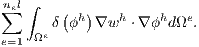
<body><![CDATA[<br>    </font>        <p> </p>         <p>   <font face="Verdana" size="2">The dimensionless stabilizations parameters are local (element level) so, the velocity modulus <img src="/img/revistas/cleiej/v15n3/3a0251x.png" alt="&#8741;&#8741; h&#8741;&#8741;  u " class="math"> is calculated for each element <img src="/img/revistas/cleiej/v15n3/3a0252x.png" alt="e  " class="math"> and <img src="/img/revistas/cleiej/v15n3/3a0253x.png" alt="&#120101;  " class="math"> is an element length measure based in its volume <img src="/img/revistas/cleiej/v15n3/3a0254x.png" alt="&#120089;  " class="math"> as shown bellow </font>    </p>     <table class="equation">       <tbody>         <tr>           <td><font face="Verdana" size="2"><a id="x1-4004r14"></a>                                       </font>                                       <center class="math-display">       <font face="Verdana" size="2">       <img src="/img/revistas/cleiej/v15n3/3a0255x.png" alt="    &#8728; --- &#120101; = 3 6&#120089;-.       &pi;" class="math-display"></font></center>           </td>           <td class="equation-label"><font face="Verdana" size="2">(14)</font></td>         </tr>                   </tbody> </table>      <font face="Verdana" size="2">          <br>    </font>        <p> <font face="Verdana" size="2">The discretized dimensionless body force are represented by <img src="/img/revistas/cleiej/v15n3/3a0256x.png" alt="lh  " class="math">.&nbsp;</font></p>         <p>   <font face="Verdana" size="2">For the dimensionless advective-diffusive transport we adopt the same assumptions, so given the following finite-dimensional trial solution and weight functions spaces for the scalar </font>    </p>     <table class="equation">       <tbody>         <tr>           <td><font face="Verdana" size="2"><a id="x1-4005r15"></a>                                       </font>                                       <center class="math-display">       <font face="Verdana" size="2">       <img src="/img/revistas/cleiej/v15n3/3a0257x.png" alt="     {                     .-h       } Sh&#981; = &#981;h | &#981;h &isin; H1h(&Omega;) , &#981;h= &#981;  in  &Gamma; &#981; , V h= {wh | wh &isin; H1h (&Omega;), wh .= 0 em &Gamma; }  w                                  &#981;" class="math-display"></font></center>           </td>           <td class="equation-label"><font face="Verdana" size="2">(15)</font></td>         </tr>                   </tbody> </table>      <font face="Verdana" size="2">          <br>    </font>        <p> <font face="Verdana" size="2">the stabilized FEM formulation can be written as: Find <img src="/img/revistas/cleiej/v15n3/3a0258x.png" alt=" h    h &#981;  &isin; S&#981;  " class="math"> such as, <img src="/img/revistas/cleiej/v15n3/3a0259x.png" alt="   h   h &forall;w  &isin; Vw  " class="math">, </font>    </p>     <table class="equation">       <tbody>         <tr>           <td><font face="Verdana" size="2"><a id="x1-4006r16"></a>                                       </font>                                       <center class="math-display">       <font face="Verdana" size="2">       <img src="/img/revistas/cleiej/v15n3/3a0260x.png" alt="&int;      (   h         )        &int;  (    )          &int;    wh &sdot; &part;-&#981;-+ uh &sdot;&nabla;&#981;h  d&Omega; + 1-    &nabla;wh T &sdot;&nabla; &#981;hd&Omega; -   whqd&Gamma; +   &Omega;      &part;t                 D  &Omega;                   &Gamma; &sum;nel &int;  (      h     h) ((&part; &#981;h   h    h) ]   e       e &tau;SUPGu  &sdot;&nabla;w   &sdot;  -&part;t-+ u  &sdot;&nabla;&#981;    d&Omega;  = 0. e=1  &Omega;" class="math-display"></font></center>           </td>           <td class="equation-label"><font face="Verdana" size="2">(16)</font></td>         </tr>                   </tbody> </table>      <font face="Verdana" size="2">          <br>    </font>        <p> </p>         ]]></body>

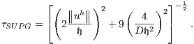
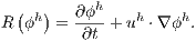
<body><![CDATA[<p>   <font face="Verdana" size="2">The three first integrals in&nbsp;(<a href="#x1-4006r16">16</a>) come from the Galerkin weak formulation. The integral into the summation over the elements is the SUPG stabilization. The non-dimensional stabilization parameter is computed similarly to&nbsp;(<a href="#x1-4003r13">13</a>), that is: </font>    </p>     <table class="equation">       <tbody>         <tr>           <td><font face="Verdana" size="2"><a id="x1-4007r17"></a>                                       </font>                                       <center class="math-display">       <font face="Verdana" size="2">       <img src="/img/revistas/cleiej/v15n3/3a0261x.png" alt="        &lfloor; ( &#8741;  &#8741; )2    (    )2&rfloor;- 12 &tau;     = &lceil;  2&#8741;uh&#8741;-  + 9  --4-  &rceil;   .  SUPG         &#120101;         D &#120101;2" class="math-display"></font></center>           </td>           <td class="equation-label"><font face="Verdana" size="2">(17)</font></td>         </tr>                   </tbody> </table>      <font face="Verdana" size="2">          <br>    </font>        <p> </p>         <p>   <font face="Verdana" size="2">In the stabilized formulations (<a href="#x1-4006r16">16</a>), an additional stabilization is added to handle instabilities in the numerical solution of flows with presence of strong gradients of the scalar being transported. In <span class="cite">(<a name="6."></a><a href="#6..">6</a>)</span> is presented a discontinuity capturing term which is calculated as follows: </font>    </p>     <table class="equation">       <tbody>         <tr>           <td><font face="Verdana" size="2"><a id="x1-4008r18"></a>                                       </font>                                       <center class="math-display">       <font face="Verdana" size="2">       <img src="/img/revistas/cleiej/v15n3/3a0262x.png" alt="n&sum;el&int;        &delta;(&#981;h)&nabla;wh &sdot;&nabla; &#981;hd&Omega;e. e=1 &Omega;e" class="math-display"></font></center>           </td>           <td class="equation-label"><font face="Verdana" size="2">(18)</font></td>         </tr>                   </tbody> </table>      <font face="Verdana" size="2">          <br>    </font>        <p> </p>         <p>   <font face="Verdana" size="2">Because the <img src="/img/revistas/cleiej/v15n3/3a0263x.png" alt="&delta;  " class="math"> parameter is a function of the scalar,&nbsp;(<a href="#x1-4006r16">16</a>) can be understood as a nonlinear diffusion operator. In this work, the <img src="/img/revistas/cleiej/v15n3/3a0264x.png" alt="&delta;  " class="math"> parameter was adapted from <span class="cite">(<a href="#6..">6</a>)</span> as follows in dimensionless form </font>    </p>     <table class="equation">       <tbody>         <tr>           <td><font face="Verdana" size="2"><a id="x1-4009r19"></a>                                       </font>                                       <center class="math-display">       <font face="Verdana" size="2">       <img src="/img/revistas/cleiej/v15n3/3a0265x.png" alt="                 (            ) &beta;&#8725;2-1  ( h)   ||1   ( h)||  &sum;3 ||1 &part;&#981;h ||2       &#120101;&beta; &delta; &#981;   = ||&#981;-*R &#981;  ||     ||&#981;*&part;xi-||       2                    i=1" class="math-display"></font></center>           </td>           <td class="equation-label"><font face="Verdana" size="2">(19)</font></td>         </tr>                   </tbody> </table>      <font face="Verdana" size="2">          <br>    </font>        <p> <font face="Verdana" size="2">where <img src="/img/revistas/cleiej/v15n3/3a0266x.png" alt=" * &#981; " class="math"> is a dimensionless value of the scalar (usually taken as 1) and <img src="/img/revistas/cleiej/v15n3/3a0267x.png" alt="  ( h) R  &#981; " class="math"> is an approximation for the actual residual defined as: </font>    </p>     <table class="equation">       <tbody>         <tr>           <td><font face="Verdana" size="2"><a id="x1-4010r20"></a>                                       </font>                                       <center class="math-display">       <font face="Verdana" size="2">       <img src="/img/revistas/cleiej/v15n3/3a0268x.png" alt=" (  )   &part;&#981;h R &#981;h  = ----+ uh &sdot;&nabla; &#981;h.          &part;t" class="math-display"></font></center>           </td>           <td class="equation-label"><font face="Verdana" size="2">(20)</font></td>         </tr>                   </tbody> </table>      <font face="Verdana" size="2">          <br>    </font>        ]]></body>
<body><![CDATA[<p> </p>         <p>   <font face="Verdana" size="2">The <img src="/img/revistas/cleiej/v15n3/3a0269x.png" alt="&beta;  " class="math"> parameter can be set as 1 or 2.&nbsp;</font></p>         <p>    </p>         <p><font face="Verdana" size="2"><span class="titlemark">2.3   </span> <a id="x1-50002.3"></a>Discretized Systems</font></p>      <font face="Verdana" size="2">          <br>    </font>        <p><font face="Verdana" size="2">Adopting the implicit backward Euler scheme for the time discretization together with a fixed point linearization, the final discrete system of&nbsp;(<a href="#x1-4002r12">12</a>) and&nbsp;(<a href="#x1-4006r16">16</a>) results in </font>    </p>     <table class="equation">       <tbody>         <tr>           <td><font face="Verdana" size="2"><a id="x1-5001r21"></a>                                       </font>                                       <center class="math-display">       <font face="Verdana" size="2">       <img src="/img/revistas/cleiej/v15n3/3a0270x.png" alt="          n+1,k+1     (  ( n+1,k)     ( n+1,k)    )  n+1,k+1 (M + M &tau;)u       + &Delta;t N  u      +N &tau; u      + K  u      - &Delta;t(G - G&tau;)pn+1,k+1 = &Delta;t (f (&#981;n )+ f&tau; (&#981;n))+ (M + M &tau;)un," class="math-display"></font></center>           </td>           <td class="equation-label"><font face="Verdana" size="2">(21)</font></td>         </tr>                   </tbody> </table>      <font face="Verdana" size="2">          <br>    </font>        <p>    </p>     <table class="equation">       <tbody>         <tr>           <td><font face="Verdana" size="2"><a id="x1-5002r22"></a>                                       </font>                                       <center class="math-display">       <font face="Verdana" size="2">       <img src="/img/revistas/cleiej/v15n3/3a0271x.png" alt="    T n+1,k+1      n+1,k+1     (  ( n+1,k) n+1,k+1      n+1,k+1) &Delta;tG  u       + M &xi;u      + &Delta;t  N&xi; u      u      + G &xi;p       = &Delta;tf&xi; (&#981;n )+ M &xi;un," class="math-display"></font></center>           </td>           <td class="equation-label"><font face="Verdana" size="2">(22)</font></td>         </tr>                   </tbody> </table>      <font face="Verdana" size="2">          <br>    </font>        <p>    </p>     <table class="equation">       <tbody>         <tr>           <td><font face="Verdana" size="2"><a id="x1-5003r23"></a>                                       </font>                                       <center class="math-display">       <font face="Verdana" size="2">       <img src="/img/revistas/cleiej/v15n3/3a0272x.png" alt=" (M  + M )&#981;n+1,k+1+    (  (&tau;   )     (    )         (      )) &Delta;t  N  un+1 + N &tau; un+1 + K + K &delta; &#981;n+1,k  &#981;n+1,k+1 =            n  (M  + M&tau;)&#981;  ." class="math-display"></font></center>           </td>           <td class="equation-label"><font face="Verdana" size="2">(23)</font></td>         </tr>                   </tbody> </table>      <font face="Verdana" size="2">          ]]></body>
<body><![CDATA[<br>    </font>        <p> </p>         <p>   <font face="Verdana" size="2">In the matrix systems&nbsp;(<a href="#x1-5001r21">21</a>),&nbsp;(<a href="#x1-5002r22">22</a>) and&nbsp;(<a href="#x1-5003r23">23</a>) <img src="/img/revistas/cleiej/v15n3/3a0273x.png" alt="u  " class="math">, <img src="/img/revistas/cleiej/v15n3/3a0274x.png" alt="p  " class="math"> and <img src="/img/revistas/cleiej/v15n3/3a0275x.png" alt="&#981; " class="math"> are the nodal vectors of the correspondent unknowns <img src="/img/revistas/cleiej/v15n3/3a0276x.png" alt="uh  " class="math">, <img src="/img/revistas/cleiej/v15n3/3a0277x.png" alt="ph  " class="math"> and <img src="/img/revistas/cleiej/v15n3/3a0278x.png" alt="&#981;h  " class="math">, and <img src="/img/revistas/cleiej/v15n3/3a0279x.png" alt="&Delta;t  " class="math"> stands for the time-step size. The super indexes <img src="/img/revistas/cleiej/v15n3/3a0280x.png" alt="n +1  " class="math"> and <img src="/img/revistas/cleiej/v15n3/3a0281x.png" alt="n  " class="math"> mean the current and previous time-steps while <img src="/img/revistas/cleiej/v15n3/3a0282x.png" alt="k+ 1  " class="math"> and <img src="/img/revistas/cleiej/v15n3/3a0283x.png" alt="k  " class="math"> are respectively the current and previous nonlinear iterations counter.&nbsp;</font></p>         <p>   <font face="Verdana" size="2">For the matrices where the advective operator appears, i.e., Galerkin advection, SUPG mass and advection, and PSPG advection, the velocity components are evaluated at each integration point. <img src="/img/revistas/cleiej/v15n3/3a0284x.png" alt="M  " class="math"> is the mass matrix, <img src="/img/revistas/cleiej/v15n3/3a0285x.png" alt="K  " class="math"> is the viscous/diffusive matrix, <img src="/img/revistas/cleiej/v15n3/3a0286x.png" alt="N (u)  " class="math"> is the nonlinear advection matrix, <img src="/img/revistas/cleiej/v15n3/3a0287x.png" alt="G  " class="math"> and <img src="/img/revistas/cleiej/v15n3/3a0288x.png" alt="GT  " class="math"> are the gradient and its transpose (divergent) matrices. <img src="/img/revistas/cleiej/v15n3/3a0289x.png" alt="f  " class="math"> is the body force vector. <img src="/img/revistas/cleiej/v15n3/3a0290x.png" alt="K  (&#981;)   &delta;  " class="math"> is the nonlinear discontinuity capturing matrix. The matrices and vectors with the subscripts <img src="/img/revistas/cleiej/v15n3/3a0291x.png" alt="&tau;  " class="math"> and <img src="/img/revistas/cleiej/v15n3/3a0292x.png" alt="&xi;  " class="math"> mean the SUPG and PSPG terms.&nbsp;</font></p>         <p>    </p>         <p><font face="Verdana" size="2"><span class="titlemark">3   </span> <a id="x1-60003"></a>Computational Aspects</font></p>      <font face="Verdana" size="2">          <br>    </font>        <p>    </p>         <p><font face="Verdana" size="2"><span class="titlemark">3.1   </span> <a id="x1-70003.1"></a>Mesh Adaptivity</font></p>      <font face="Verdana" size="2">          <br>    </font>        ]]></body>
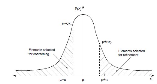
<body><![CDATA[<p><font face="Verdana" size="2">The mesh adaptivity together with high-performance computing (parallel processing) play a key role to enable numerical simulations of actual engineering/industrial problems within an acceptable time without exhausting the processing capacity of current computers.&nbsp;</font></p>         <p>   <font face="Verdana" size="2">Particularly for the density current problem, AMR/C is a important tool to capture and track the flow structure at the front, where the Kelvin-Helmholtz billows occur. From an initial coarse mesh, the adaptivity refinement process begins near the interface between the two fluids and it follows its development.&nbsp;</font></p>         <p>   <font face="Verdana" size="2">In <span class="obeylines-h"><span class="verb"><span class="cmtt-10">libMesh</span></span></span> the mesh refinement can be accomplished by element subdivision (h-refinement), increasing the local polynomial degree (p-refinement) as well a combination of both methods (hp-refinement). Although there is an extensive literature devoted to obtaining reliable a posteriori estimators that are more closely linked to the operators and governing equations <span class="cite">(<a name="7."></a><a href="#7..">7</a>,&nbsp;<a name="8."></a><a href="#8..">8</a>)</span>, in <span class="obeylines-h"><span class="verb"><span class="cmtt-10">libMesh</span></span></span> the error indicator is focused on local indicators that are essentially independent of the physics <span class="cite">(<a href="#XKirk06">2</a>)</span>.&nbsp;</font></p>         <p>   <font face="Verdana" size="2">   <span class="obeylines-h"><span class="verb"><span class="cmtt-10">libMesh</span></span></span> uses a statistical refinement/coarsening scheme based on the ideas presented in <span class="cite">(<a name="9."></a><a href="#9..">9</a>)</span> where the mean <img src="/img/revistas/cleiej/v15n3/3a0293x.png" alt="&mu;  " class="math"> and the standard deviation <img src="/img/revistas/cleiej/v15n3/3a0294x.png" alt="&sigma;  " class="math"> of the error indicator &ldquo;population&rdquo; are computed. Using refinement and coarsening fractions (<img src="/img/revistas/cleiej/v15n3/3a0295x.png" alt="rf  " class="math"> and <img src="/img/revistas/cleiej/v15n3/3a0296x.png" alt="rc  " class="math">), the elements are flagged for refinement and coarsening as showed in Fig.&nbsp;(<a href="#x1-70011">1</a>).&nbsp;</font></p>         <p>   </p>     <hr class="float">     <div class="float">      <div class="centerline">                                              <font face="Verdana" size="2">                                           <a id="x1-70011"><img src="/img/revistas/cleiej/v15n3/3a02f1.jpg" alt="PIC"></a>   </font> </div>      <font face="Verdana" size="2">          <br>       </font>           <div class="caption"><font face="Verdana" size="2"><span class="id">Figure&nbsp;1: </span><span class="content">Statistical refinement: elements in hatched areas are flagged to AMR/C process</span></font></div>     <font face="Verdana" size="2">         <br>        </font>        </div>     <hr class="endfloat"> <font face="Verdana" size="2">     ]]></body>
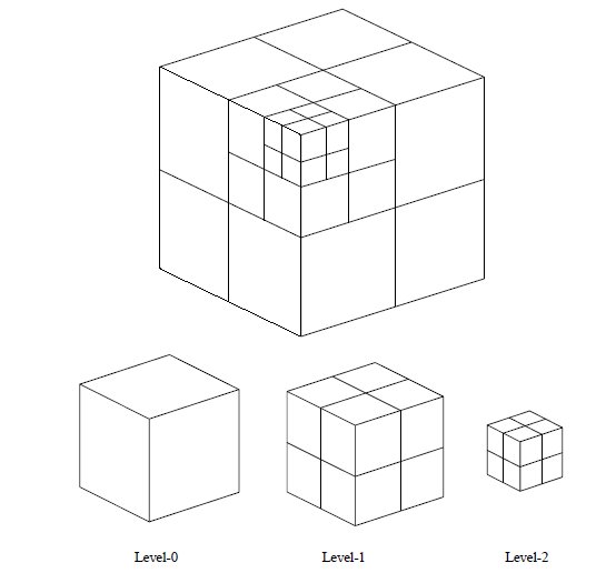
<body><![CDATA[<br>    </font>        <p>   <font face="Verdana" size="2">This scheme is suitable for evolution problems where, in the beginning, a small error is evenly distributed. Throughout the simulation the error distribution spreads and the AMR/C process starts. Whether the solution approaches its steady-state, the distribution of error also reaches the steady-state, stopping the AMR/C process.&nbsp;</font></p>         <p>   <font face="Verdana" size="2">The elements are refined through a &ldquo;natural refinement&rdquo; scheme: elements of dimension <img src="/img/revistas/cleiej/v15n3/3a0297x.png" alt="d  " class="math">, with the exception of the pyramids, produce <img src="/img/revistas/cleiej/v15n3/3a0298x.png" alt="2d  " class="math"> elements of the same type after refinement. The degrees of freedom are constrained at the hanging nodes on element interfaces. This approach yields a tree data structure formed by the &ldquo;parents&rdquo; and their &ldquo;children&rdquo; elements. An example of an element level hierarchy resulting from the application of this scheme for a hexahedral mesh is presented in Fig.&nbsp;<a href="#x1-70022">2</a>.&nbsp;</font></p>         <p>   </p>     <hr class="float">     <div class="float">      <div class="centerline">                 <font face="Verdana" size="2">                 <a id="x1-70022"><img src="/img/revistas/cleiej/v15n3/3a02f2.jpg" alt="PIC"></a> </font> </div>      <font face="Verdana" size="2">          <br>       </font>           <div class="caption"><font face="Verdana" size="2"><span class="id">Figure&nbsp;2: </span><span class="content">Hierarchy levels of the refinement of an hexahedral element</span></font></div>     <font face="Verdana" size="2">         <br>        </font>        </div>     <hr class="endfloat"> <font face="Verdana" size="2">     <br>    </font>        ]]></body>
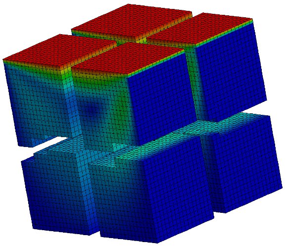
<body><![CDATA[<p>   <font face="Verdana" size="2">The elements present in the initial mesh (level-0 elements) have no parents as well the active elements (those that are part of the current simulation mesh) have no children, so the latter are the current high-level elements. The element level is determined recursively from its parents and the user should determine the maximum refinement level.&nbsp;</font></p>         <p>   <font face="Verdana" size="2">The frequency of refinement/coarsening is an user&rsquo;s responsibility. When the mesh adapts it is optimized for the state at the current time <span class="cite">(<a name="10."></a><a href="#10..">10</a>)</span>. One should find a frequency of adaptivity which will balance the computational effort and quality of results as there is a computational cost associated with the adaptivity process. When the mesh is adapted, the field solution should be projected (interpolated) and a simulation should be performed on the new mesh.&nbsp;</font></p>         <p>   <font face="Verdana" size="2">In this work we use a class of errors estimators based on derivative jump (or flux jump) of the transported scalar calculated at the elements interface called Kelly&rsquo;s Error Estimator <span class="cite">(<a name="11."></a><a href="#11..">11</a>)</span> to perform the h-refinement. The refinement and coarsening fractions for the statistical strategy as well the adaptivity frequency are set independently for each simulation problem. </font>    </p>         <p><font face="Verdana" size="2"><span class="titlemark">3.2   </span> <a id="x1-80003.2"></a>Domain Decomposition</font></p>      <font face="Verdana" size="2">          <br>    </font>        <p><font face="Verdana" size="2">In this paper, we consider the standard partitioning domain without overlap, as shown in Fig.&nbsp;(<a href="#x1-80013">3</a>), where the elements related to each of the sub-domains are assigned to different processors. That is, the simulation domain <img src="/img/revistas/cleiej/v15n3/3a0299x.png" alt="&Omega;h  " class="math"> is divided into a discrete set of sub-domains <img src="/img/revistas/cleiej/v15n3/3a02100x.png" alt="&Omega;hp  " class="math"> such as <img src="/img/revistas/cleiej/v15n3/3a02101x.png" alt="&#8899; &Omega;hp = &Omega;h  " class="math"> and <img src="/img/revistas/cleiej/v15n3/3a02102x.png" alt="&#8898;&Omega;hp = &empty; " class="math">.&nbsp;</font></p>         <p>   </p>     <hr class="float">     <div class="float">      <div class="centerline">                                              <font face="Verdana" size="2">                                           <a id="x1-80013"><img src="/img/revistas/cleiej/v15n3/3a02f3.jpg" alt="PIC"></a>   </font> </div>      <font face="Verdana" size="2">          <br>       </font>           ]]></body>
<body><![CDATA[<div class="caption"><font face="Verdana" size="2"><span class="id">Figure&nbsp;3: </span><span class="content">Simulation domain decomposition in 8 sub-domains</span></font></div>     <font face="Verdana" size="2">         <br>        </font>        </div>     <hr class="endfloat"> <font face="Verdana" size="2">     <br>    </font>        <p>   <font face="Verdana" size="2">In AMR/C computations at a new adaptation stage, regions of the domain will have an increase in mesh element density while in others, the number of elements will decrease. These dynamic mesh adjustments result for some processors in significant increasing (or decreasing) work therefore causing load unbalancing <span class="cite">(<a href="#XDongarra03">1</a>)</span>.&nbsp;</font></p>         <p>   <font face="Verdana" size="2">Libraries such as METIS and ParMETIS were developed aiming implementing efficient partitioning mesh schemes. The first is a serial mesh partitioning library, while the second is based on parallel MPI. Both can also reorder the unknowns in unstructured grids to minimize the fill-in during LU factorization. The ParMETIS extends the functionality provided by METIS and includes routines for parallel computations with adaptive meshes refinement and large-scale numerical simulations. </font>    </p>         <p><font face="Verdana" size="2"><span class="titlemark">3.3   </span> <a id="x1-90003.3"></a>Parallel Solution of Preconditioned Linear Systems</font></p>      <font face="Verdana" size="2">          <br>    </font>        <p><font face="Verdana" size="2">The support for the numerical solution of the resulting system of linear equations in the parallel architecture environment is provided by PETSc. It provides structures for efficient storage (vectors, arrays, for example), as well ways to handle it. The <span class="obeylines-h"><span class="verb"><span class="cmtt-10">libMesh</span></span></span> uses compressed sparse row (CSR) data structure to store the sparse matrices. PETSc has a number of methods for solving linear sparse system as GMRES and BiConjugate Gradient method (BiCG) and several types of preconditioners as ILU(k) and Block-Jacobi. Options for reordering the linear system as the Reverse Cuthill-McKee method (RCM, <span class="cite">(<a name="12."></a><a href="#12..">12</a>)</span>) are also available.&nbsp;</font></p>         <p>   <font face="Verdana" size="2">In this work we use Block-Jacobi sub-domain preconditioning. It is one of the most widely used schemes due to its easiness of implementation. There are no overlap between the blocks. The incomplete factorization may be applied to each of them without extra communication costs. However, in adaptive simulations, the new local factorization should be performed every time the mesh is modified since the adaptivity changes the group of elements residing in each sub-domain <span class="cite">(<a name="13."></a><a href="#13..">13</a>)</span>. It is usual to refer to the Block-Jabobi preconditioning strategy in conjunction with the ILU factorization with a certain level <img src="/img/revistas/cleiej/v15n3/3a02103x.png" alt="k  " class="math"> of fill-in by BILU(<img src="/img/revistas/cleiej/v15n3/3a02104x.png" alt="k  " class="math">) <span class="cite">(<a name="14."></a><a href="#14..">14</a>)</span>.&nbsp;</font></p>         <p>   <font face="Verdana" size="2">The communication between the processors, such as required for the algebraic operations or during assembly of arrays of elements are supported by a set of PETSc library routines which is designed for parallel computing using the MPI API.&nbsp;</font></p>         ]]></body>
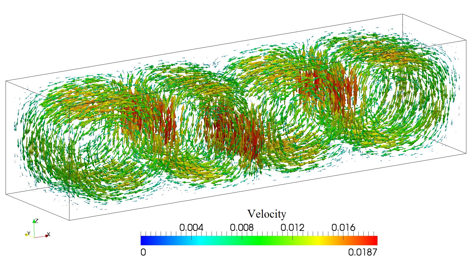
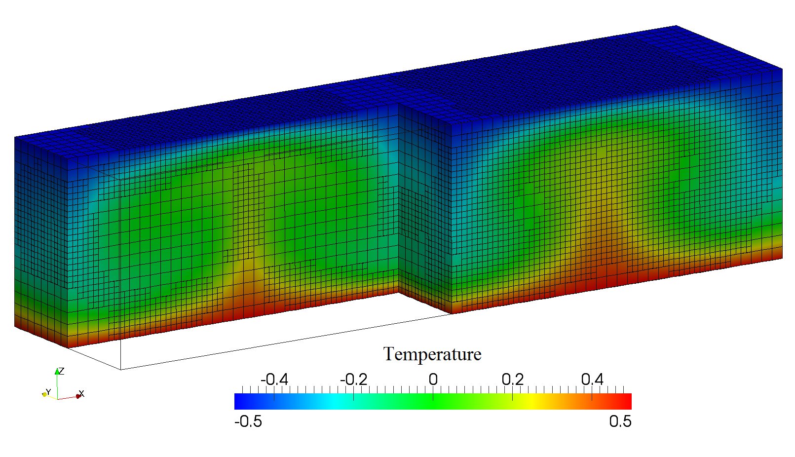
<body><![CDATA[<p>    </p>         <p><font face="Verdana" size="2"><span class="titlemark">4   </span> <a id="x1-100004"></a>Numerical Results</font></p>      <font face="Verdana" size="2">          <br>    </font>        <p><font face="Verdana" size="2">The simulations were performed in a SGI Altix ICE 8400 cluster with 640 cores (Intel Nehalem). This machine has 1.28 TB of distributed memory. The processing nodes are connected by InfiniBand. The cluster is located at the High-Performance Computing Center (NACAD) of the Federal University of Rio de Janeiro, Brazil.&nbsp;</font></p>         <p>    </p>         <p><font face="Verdana" size="2"><span class="titlemark">4.1   </span> <a id="x1-110004.1"></a>Parallel Adaptive Simulation of the Rayleigh-B&eacute;nard Problem</font></p>      <font face="Verdana" size="2">          <br>    </font>        <p><font face="Verdana" size="2">In this example we consider the Rayleigh-B&eacute;nard natural convection in a container with geometric domain <img src="/img/revistas/cleiej/v15n3/3a02105x.png" alt="&Omega; = (0,4]&times; (0,1]&times; (0,1)  " class="math">. This problem consists to solve a natural convection phenomenon of a fluid which initially at rest (<img src="/img/revistas/cleiej/v15n3/3a02106x.png" alt="t = 0  " class="math">) produces a sequence of adjacent convection cells along the longitudinal direction (<img src="/img/revistas/cleiej/v15n3/3a02107x.png" alt="x  " class="math"> axis) due to the temperature difference between its upper (cold) and lower (hot) walls.&nbsp;</font></p>         <p>   <font face="Verdana" size="2">No-slip boundary conditions are imposed in all the walls and the pressure is prescribed as <img src="/img/revistas/cleiej/v15n3/3a02108x.png" alt="p(2.0,0.5,0.0) = 0.0  " class="math">. The dimensionless cold temperature is <img src="/img/revistas/cleiej/v15n3/3a02109x.png" alt="Tc = - 0.5  " class="math"> and the hot <img src="/img/revistas/cleiej/v15n3/3a02110x.png" alt="Th = 0.5  " class="math">. The physical problem is defined setting the Reynolds Number as <img src="/img/revistas/cleiej/v15n3/3a02111x.png" alt="Re = 4,365  " class="math">, Grashof number as <img src="/img/revistas/cleiej/v15n3/3a02112x.png" alt="Gr = 41,666.66  " class="math">, the Peclet number as <img src="/img/revistas/cleiej/v15n3/3a02113x.png" alt="P e = 3,142.8  " class="math"> and Froude number (besides not introduced in the Navier-Stokes equations presented in section <a href="#x1-30002.1">2.1</a>, the Froude number is used here to take into account the fluid&rsquo;s weight in the calculation. More details about how to incorporate the Froude number in the dimensionless Navier-Stokes equations may be found in <span class="cite">(<a href="#3..">3</a>)</span>.) as <img src="/img/revistas/cleiej/v15n3/3a02114x.png" alt="F r = 0.6432  " class="math">.&nbsp;</font></p>         <p>   <font face="Verdana" size="2">Only one refinement/coarsening level was allowed at every 25 time-steps. For the statistical adaptivity scheme the refinement fraction is <img src="/img/revistas/cleiej/v15n3/3a02115x.png" alt="rf = 0.6  " class="math"> and coarsening fraction is <img src="/img/revistas/cleiej/v15n3/3a02116x.png" alt="rc = 0.01  " class="math">. The linear tolerance for GMRES(30) together with the BILU(<img src="/img/revistas/cleiej/v15n3/3a02117x.png" alt="1  " class="math">) and reordering by RCM method is <img src="/img/revistas/cleiej/v15n3/3a02118x.png" alt="       -6 1.0&times; 10  " class="math">. The nonlinear tolerance is <img src="/img/revistas/cleiej/v15n3/3a02119x.png" alt="      - 5 1.0 &times; 10  " class="math"> and the constant time step size is <img src="/img/revistas/cleiej/v15n3/3a02120x.png" alt="&Delta;t = 5.0  " class="math">.&nbsp;</font></p>         ]]></body>

<body><![CDATA[<p>   <font face="Verdana" size="2">The steady-state velocity vectors are shown in Fig.(<a href="#x1-110014">4</a>) and the temperature over the final adapted mesh is plotted in Fig.(<a href="#x1-110025">5</a>).&nbsp;</font></p>         <p>   </p>     <hr class="float">     <div class="float">  <font face="Verdana" size="2">      <br>       </font>           <div class="caption"><font face="Verdana" size="2"><a id="x1-110014" href="/img/revistas/cleiej/v15n3/3a02f4.jpg"> <span class="id">Figure&nbsp;4: </span><span class="content">Steady-state velocity vectors</span></a></font></div>     <font face="Verdana" size="2">         <br>          </font>          </div>     <hr class="endfloat">  <font face="Verdana" size="2">      <br>     </font>         <p>   </p>     <hr class="float">     <div class="float">  <font face="Verdana" size="2">      <br>       </font>           ]]></body>
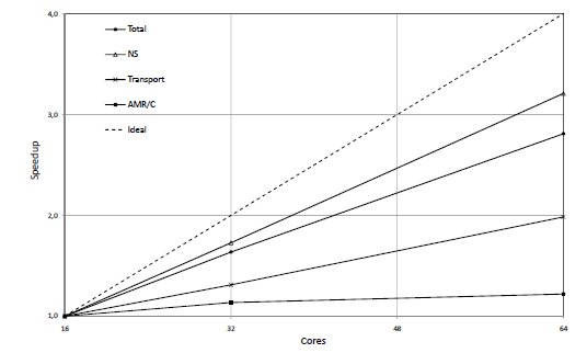
<body><![CDATA[<div class="caption"> <font face="Verdana" size="2"> <a id="x1-110025" href="/img/revistas/cleiej/v15n3/3a02f5.jpg"><span class="id">Figure&nbsp;5: </span><span class="content">Temperature at steady-state and final adapted mesh</span></a></font></div>      <font face="Verdana" size="2">          <br>          </font>          </div>     <hr class="endfloat"> <font face="Verdana" size="2">     <br>     </font>         <p>   <font face="Verdana" size="2">The Fig. (<a href="#x1-110046">6</a>) presents the speedup for the total simulation time, the total time for solving the Navier-Stokes and transport problems and the AMR/C procedure considering in the numerator the time spent with 16 CPU&rsquo;s, i.e., </font>    </p>     <table class="equation">       <tbody>         <tr>           <td><font face="Verdana" size="2"><a id="x1-11003r24"></a>                                       </font>                                       <center class="math-display">       <font face="Verdana" size="2">       <img src="/img/revistas/cleiej/v15n3/3a02121x.png" alt="     &tau; Sp = -16.       &tau;p" class="math-display"></font></center>           </td>           <td class="equation-label"><font face="Verdana" size="2">(24)</font></td>         </tr>                   </tbody> </table>      <font face="Verdana" size="2">          <br>    </font>        <p>  </p>         <p>   </p>     <hr class="float">     <div class="float">      <div class="centerline"> <font face="Verdana" size="2"> <a id="x1-110046"><img src="/img/revistas/cleiej/v15n3/3a02f6.jpg" alt="PIC"></a> </font> </div>      <font face="Verdana" size="2">          <br>       </font>           ]]></body>
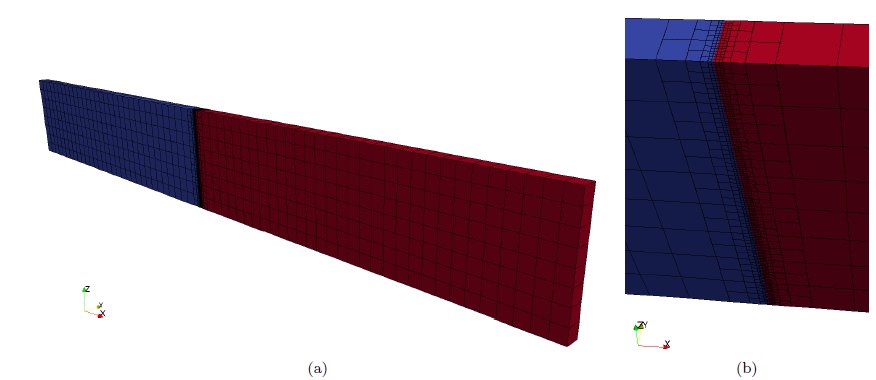
<body><![CDATA[<div class="caption"><font face="Verdana" size="2"><span class="id">Figure&nbsp;6: </span><span class="content">Speedup for the Rayleigh-B&eacute;nard problem</span></font></div>     <font face="Verdana" size="2">         <br>        </font>        </div>     <hr class="endfloat"> <font face="Verdana" size="2">     <br>    </font>        <p>   <font face="Verdana" size="2">The AMR/C time does not reach <img src="/img/revistas/cleiej/v15n3/3a02122x.png" alt="10%  " class="math"> of the total simulation time. We may observe from the results of Fig.(<a href="#x1-110046">6</a>) that the present simulation achieves a good parallel performance, that is, speed up around 3 for the total simulation with 64-cores run with respect to 16-cores run (over 3 for the Navier-Stokes simulation).&nbsp;</font></p>         <p>   <font face="Verdana" size="2">Despite the good overall performance, it is observed that the adaptive procedure does not scale as well as the linear solvers (<img src="/img/revistas/cleiej/v15n3/3a02123x.png" alt="S64 = 1.22)  " class="math">. The poor performance of the AMR/C procedure in the current <span class="obeylines-h"><span class="verb"><span class="cmtt-10">libMesh</span></span></span> release is due to the fact that all mesh data are replicated on all cores, which increases memory requirements and communication per core. </font>    </p>         <p><font face="Verdana" size="2"><span class="titlemark">4.2   </span> <a id="x1-120004.2"></a>Temperature-driven gravity current with AMR/C</font></p>      <font face="Verdana" size="2">          <br>    </font>        <p><font face="Verdana" size="2">For the simulation of a temperature-driven gravity current with mesh adaptivity, we consider a slice domain (to emulate a 2D simulation domain from a mesh composed of 3D elements, the slice domain is positioned parallel to the <img src="/img/revistas/cleiej/v15n3/3a02124x.png" alt="xz  " class="math"> plane and the perpendicular direction <img src="/img/revistas/cleiej/v15n3/3a02125x.png" alt="(0,y,0)  " class="math"> is discretized with only one element except at regions where the mesh adapts. For all nodes on the mesh <img src="/img/revistas/cleiej/v15n3/3a02126x.png" alt="vy = 0.0  " class="math"> is imposed.) <img src="/img/revistas/cleiej/v15n3/3a02127x.png" alt="&Omega; = (0,L )&times; (0,H &#8725;8)&times; (0,H)  " class="math"> where the nondimensional length and height are <img src="/img/revistas/cleiej/v15n3/3a02128x.png" alt="L = 0.8  " class="math"> and <img src="/img/revistas/cleiej/v15n3/3a02129x.png" alt="H = 0.1  " class="math">. The left half of the channel is initially filled with the cold fluid and the right half is filled with hot fluid. The Fig. (<a href="#x1-120017">7</a>) shows the initial configuration and a detail of the refinement at the center of the domain.&nbsp;</font></p>         <p>   </p>     <hr class="figure">     <div class="figure"> <font face="Verdana" size="2">     ]]></body>
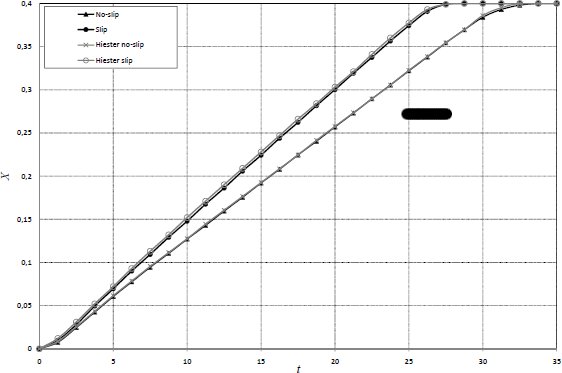
<body><![CDATA[<br>    </font>        <p><font face="Verdana" size="2"><a id="x1-120017"><img src="/img/revistas/cleiej/v15n3/3a02f7.jpg" alt="PIC"></a>     <br>      </font>      </p>         <div class="caption"><font face="Verdana" size="2"><span class="id">Figure&nbsp;7: </span><span class="content">Initial lock-exchange configuration: (a) View of the slice domain and (b) Mesh detail</span></font></div>     <font face="Verdana" size="2">         <br>   &nbsp; </font>     <p>   </p>     </div>     <hr class="endfigure"> <font face="Verdana" size="2">     <br>    </font>        <p>   <font face="Verdana" size="2">The dimensionless cold temperature is set to <img src="/img/revistas/cleiej/v15n3/3a02130x.png" alt="Tc = - 0.5  " class="math"> and the hot <img src="/img/revistas/cleiej/v15n3/3a02131x.png" alt="Th = 0.5  " class="math">. We consider no-slip boundary conditions on the bottom, left and right walls. Free-slip boundary conditions are imposed on the top one. Thus free and no slip fronts may be considered in the same simulation.&nbsp;</font></p>         <p>   <font face="Verdana" size="2">We do not consider the reduced gravity for the definitions for the dimensionless parameters and set the Reynolds number as <img src="/img/revistas/cleiej/v15n3/3a02132x.png" alt="Re = 1.0&times; 106  " class="math"> and the Grashof is set to <img src="/img/revistas/cleiej/v15n3/3a02133x.png" alt="Gr = 1.0&times; 1010  " class="math">. For this simulation, we disregard the diffusion term of the transport equation&nbsp;(<a href="#x1-3003r3">3</a>). So, the Peclet number does not need to be defined. We set the exponent of the nonlinear diffusion operator&nbsp;(<a href="#x1-4009r19">19</a>) as <img src="/img/revistas/cleiej/v15n3/3a02134x.png" alt="&beta; = 1  " class="math"> and the time step is set to <img src="/img/revistas/cleiej/v15n3/3a02135x.png" alt="&Delta;t = 0.025  " class="math">.&nbsp;</font></p>         <p>   <font face="Verdana" size="2">We compare the results from the present adaptive simulation with those obtained using fixed structured mesh with characteristic length <img src="/img/revistas/cleiej/v15n3/3a02136x.png" alt="l = 0.00078125  " class="math"> (given by the hexahedron edge). The dimensionless distance of the front head between the two fluids <img src="/img/revistas/cleiej/v15n3/3a02137x.png" alt="X = |x- 0.4| " class="math"> is tracked over time <img src="/img/revistas/cleiej/v15n3/3a02138x.png" alt="t  " class="math">. The distance from the initial position (<img src="/img/revistas/cleiej/v15n3/3a02139x.png" alt="x = 0.4  " class="math">) of both fronts using the fixed mesh is plotted in Fig.&nbsp;(<a href="#x1-120028">8</a>)&nbsp;</font></p>         ]]></body>


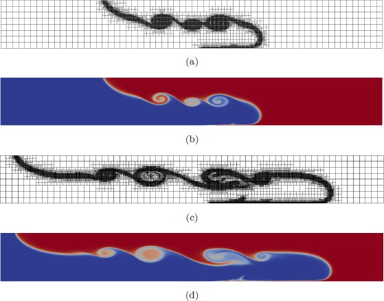
<body><![CDATA[<p>   </p>     <hr class="float">     <div class="float">     <div class="centerline">                                              <font face="Verdana" size="2">                                           <a id="x1-120028"><img src="/img/revistas/cleiej/v15n3/3a02f8.jpg" alt="PIC"> </a></font></div>      <font face="Verdana" size="2">          <br>       </font>           <div class="caption"><font face="Verdana" size="2"><span class="id">Figure&nbsp;8: </span><span class="content">Plot of the dimensionless distance of top and bottom fronts</span></font></div>     <font face="Verdana" size="2">         <br>        </font>        </div>     <hr class="endfloat"> <font face="Verdana" size="2">     <br>    </font>        <p>   <font face="Verdana" size="2">As expected, free-slip front (top) reaches the vertical wall before the no-slip (bottom) does. Figure&nbsp;(<a href="#x1-120028">8</a>) shows a good agreement between our results and those obtained by the reference <span class="cite">(<a href="#10..">10</a>)</span>. The results from <span class="cite">(<a href="#10..">10</a>)</span> were obtained using a fixed 2D mesh formed by triangles which characteristic length is <img src="/img/revistas/cleiej/v15n3/3a02140x.png" alt="l = 0.00025  " class="math">.&nbsp;</font></p>         <p>   <font face="Verdana" size="2">The Fig.&nbsp;(<a href="#x1-120039">9</a>) shows the temperature distributions and the meshes at two different times with AMR/C at every 10 time-steps. The refinement fraction is set as <img src="/img/revistas/cleiej/v15n3/3a02141x.png" alt="rf = 0.95  " class="math"> and the coarsening fraction is <img src="/img/revistas/cleiej/v15n3/3a02142x.png" alt="rc = 0.01  " class="math">. In order to prevent the size of the elements become too small, we allowed only 4 refinement-levels. The Kelvin-Helmholtz billows are captured by the mesh as the front evolves after the release.&nbsp;</font></p>         <p>   </p>     <hr class="figure">     ]]></body>
<body><![CDATA[<div class="figure">  <font face="Verdana" size="2">      <br>    </font>        <p><font face="Verdana" size="2"><a id="x1-120039"><img src="/img/revistas/cleiej/v15n3/3a02f9.jpg" alt="PIC"></a>     <br>      </font>      </p>         <div class="caption"><font face="Verdana" size="2"><span class="id">Figure&nbsp;9: </span><span class="content">Adaptive meshes and temperature distribution: (a) Adaptive mesh at <img src="/img/revistas/cleiej/v15n3/3a02143x.png" alt="t = 12.5  " class="math">, (b) Temperature distribution at <img src="/img/revistas/cleiej/v15n3/3a02144x.png" alt="t = 12.5  " class="math">, (c) Adaptive mesh at <img src="/img/revistas/cleiej/v15n3/3a02145x.png" alt="t = 25.0  " class="math"> and (d) Temperature distribution at <img src="/img/revistas/cleiej/v15n3/3a02146x.png" alt="t = 25.0  " class="math"></span></font></div>     <font face="Verdana" size="2">         <br>   &nbsp; </font>     <p>   </p>     </div>     <hr class="endfigure"> <font face="Verdana" size="2">     <br>    </font>        <p>   <font face="Verdana" size="2">Through the mesh adaptivity simulation, the largest number of elements reached is approximately 30,000. If a fixed structured mesh had been used, to achieve the same refinement level, it would take approximately 131,000 hexaedrons. Therefore, with mesh adaptation we can, in this problem, compute a solution with one order of magnitude less elements without compromising the solution accuracy. </font>    </p>         <p><font face="Verdana" size="2"><span class="titlemark">5   </span> <a id="x1-130005"></a>Conclusions</font></p>      <font face="Verdana" size="2">          ]]></body>
<body><![CDATA[<br>    </font>        <p><font face="Verdana" size="2">The <span class="obeylines-h"><span class="verb"><span class="cmtt-10">libMesh</span></span></span> framework was used to implement the stabilized SUPG/PSPG finite element formulation for the parallel adaptive solution of incompressible viscous flow and advective-diffusive transport using a trilinear hexahedral element. Good numerical results were obtained for parallel executions with adaptive meshes. AMR/C allows the representation of multiple flow scales and improves resolution where needed. It was possible to track the Kelvin-Helmholtz billows present in the temperature-driven gravity current problem.&nbsp;</font></p>         <p>    </p>         <p><font face="Verdana" size="2"><a id="x1-140005"></a>Acknowledgment</font></p>      <font face="Verdana" size="2">          <br>    </font>        <p><font face="Verdana" size="2">This work is partially supported by CNPq and ANP. We are also indebted to Engineering Simulation and Scientific Software (ESSS) to their partial support to A. Rossa in his PhD studies at COPPE/UFRJ. Computer time for the simulations in this work was provided by the High Performance Computing Center at COPPE/UFRJ.&nbsp;</font></p>         <p>    </p>         <p><font face="Verdana" size="2"><a id="x1-150005"></a>References</font></p>      <font face="Verdana" size="2">          <br>     </font>         <p>     </p>         ]]></body>
<body><![CDATA[<div class="thebibliography">          <!-- ref --><p><font face="Verdana" size="2"><span class="biblabel"><a name="1.."></a>   (<a href="#1.">1</a>)<span class="bibsp">&nbsp;&nbsp;&nbsp;</span></span>J.&nbsp;Dongarra, I.&nbsp;Foster, G.&nbsp;Fox, W.&nbsp;Gropp, K.&nbsp;Kennedy, L.&nbsp;Torczon, and A.&nbsp;White, <span class="cmti-10">Sourcebook of</span>     <span class="cmti-10">Parallel Computing</span>.   San Francisco, CA, USA: Morgan Kaufmann Publishers, 2003.     </font>     </p>               <p><font face="Verdana" size="2"><span class="biblabel"><a name="2.."></a>   (<a href="#2.">2</a>)<span class="bibsp">&nbsp;&nbsp;&nbsp;</span></span>B.&nbsp;S. Kirk, J.&nbsp;W. Peterson, R.&nbsp;H. Stogner, and G.&nbsp;F. Carey, &ldquo;<span class="cmtt-10">libMesh</span>: A C++ Library for Parallel     Adaptive Mesh Refinement/Coarsening Simulations,&rdquo; <span class="cmti-10">Engineering with Computers</span>, vol.&nbsp;22, no. 3&ndash;4,     pp. 237&ndash;254, Nov. 2006, <a href="http://dx.doi.org/10.1007/s00366-006-0049-3" class="url">http://dx.doi.org/10.1007/s00366-006-0049-3</a>. </font>     </p>               <!-- ref --><p><font face="Verdana" size="2"><span class="biblabel">   (<a name="3.."></a><a href="#3.">3</a>)<span class="bibsp">&nbsp;&nbsp;&nbsp;</span></span>M.&nbsp;Griebel,  T.&nbsp;Dornseifer,  and  T.&nbsp;Neuhoeffer,  <span class="cmti-10">Numerical  Simulation  in  Fluid  Dynamics:  A</span>     <span class="cmti-10">Practical Introduction</span>.   Philadelphia, PA, USA: SIAM, 1997.     </font>     </p>               <p><font face="Verdana" size="2"><span class="biblabel"><a name="4.."></a>   (<a href="#4.">4</a>)<span class="bibsp">&nbsp;&nbsp;&nbsp;</span></span>C.&nbsp;H&auml;rtel, E.&nbsp;Meiburg, and F.&nbsp;Necker, &ldquo;Analysis and direct numerical simulation of the flow at a     gravity-current head. Part 1. Flow topology and front speed for slip and no-slip boundaries,&rdquo; <span class="cmti-10">Journal</span>     <span class="cmti-10">of Fluid Mechanics</span>, vol. 418, pp. 189&ndash;212, Apr. 2000. </font>     </p>               <p><font face="Verdana" size="2"><span class="biblabel"><a name="5.."></a>   (<a href="#5.">5</a>)<span class="bibsp">&nbsp;&nbsp;&nbsp;</span></span>T.&nbsp;Tezduyar, &ldquo;Stabilized finite element formulations for incompressible flow computations,&rdquo; ser.     Advances in Applied Mechanics, J.&nbsp;W. Hutchinson and T.&nbsp;Y. Wu, Eds.   Elsevier, 1991, vol.&nbsp;28, pp. 1     &ndash; 44. (Online). Available: <a href="http://www.sciencedirect.com/science/article/pii/S0065215608701534" class="url">http://www.sciencedirect.com/science/article/pii/S0065215608701534</a> </font>      </p>               <p><font face="Verdana" size="2"><span class="biblabel"><a name="6.."></a>   (<a href="#6.">6</a>)<span class="bibsp">&nbsp;&nbsp;&nbsp;</span></span>Y.&nbsp;Bazilevs,   V.&nbsp;Calo,   T.&nbsp;Tezduyar,   and   T.&nbsp;Hughes,   &ldquo;<span class="cmti-10">YZ</span>&beta;  discontinuity   capturing   for     advection-dominated processes with application to arterial drug delivery,&rdquo; <span class="cmti-10">International Journal for</span>     <span class="cmti-10">Numerical Methods in Fluids</span>, vol.&nbsp;54, pp. 593&ndash;608, 2007. </font>     </p>               <p><font face="Verdana" size="2"><span class="biblabel"><a name="7.."></a>   (<a href="#7.">7</a>)<span class="bibsp">&nbsp;&nbsp;&nbsp;</span></span>R.&nbsp;E. Bank and B.&nbsp;D. Welfert, &ldquo;A posteriori error estimates for the Stokes problem,&rdquo; <span class="cmti-10">Journal on</span>     <span class="cmti-10">Numerical Analysis</span>, vol.&nbsp;28, pp. 591&ndash;623, Jun. 1991. </font>     </p>               ]]></body>
<body><![CDATA[<!-- ref --><p><font face="Verdana" size="2"><span class="biblabel"><a name="8.."></a>   (<a href="#8.">8</a>)<span class="bibsp">&nbsp;&nbsp;&nbsp;</span></span>M.&nbsp;Ainsworth    and    J.&nbsp;Oden,    <span class="cmti-10">A    Posteriori    Error    Estimation    in    Finite    Element</span>     <span class="cmti-10">Analysis</span>,    ser.    Pure    and    Applied    Mathematics.     Wiley,    2000.    (Online).    Available:     <a href="http://books.google.com.br/books?id=%5C_HligpOKcjoC" class="url">http://books.google.com.br/books?id=<span class="cmsy-10">\</span>_HligpOKcjoC</a> </font>     <!-- ref --><p><font face="Verdana" size="2"><span class="biblabel"><a name="9.."></a>   (<a href="#9.">9</a>)<span class="bibsp">&nbsp;&nbsp;&nbsp;</span></span>G.&nbsp;Carey,  <span class="cmti-10">Computational  Grids:  Generations,  Adaptation  &amp;  Solution  Strategies</span>,  ser.  Series  in     Computational and Physical Processes in Mechanics and Thermal sciEnces.   Taylor &amp; Francis, 1997.     (Online). Available: <a href="http://books.google.com.br/books?id=0w4iXh4FXKYC" class="url">http://books.google.com.br/books?id=0w4iXh4FXKYC</a> </font>     <p><font face="Verdana" size="2"><span class="biblabel"><a name="10.."></a>  (<a href="#10.">10</a>)<span class="bibsp">&nbsp;&nbsp;&nbsp;</span></span>H.&nbsp;Hiester, M.&nbsp;Piggott, and P.&nbsp;Allison, &ldquo;The impact of mesh adaptivity on the gravity current     front speed in a two-dimensional lock-exchange,&rdquo; <span class="cmti-10">Ocean Modelling</span>, vol.&nbsp;38, no. 1 - 2, pp. 1 &ndash; 21, Jan.     2011. (Online). Available: <a href="http://www.sciencedirect.com/science/article/pii/S1463500311000060" class="url">http://www.sciencedirect.com/science/article/pii/S1463500311000060</a> </font>     </p>               <p><font face="Verdana" size="2"><span class="biblabel"><a name="11.."></a>  (<a href="#11.">11</a>)<span class="bibsp">&nbsp;&nbsp;&nbsp;</span></span>D.&nbsp;W. Kelly, J.&nbsp;P. De&nbsp;S. R.&nbsp;Gago, O.&nbsp;C. Zienkiewicz, and I.&nbsp;Babuska, &ldquo;A posteriori error analysis and adaptive processes in the finite element method: Part I - Error analysis,&rdquo; <span class="cmti-10">International Journal</span>     <span class="cmti-10">for Numerical Methods in Engineering</span>, vol.&nbsp;19, no.&nbsp;11, pp. 1593&ndash;1619, Nov. 1983. (Online). Available:     <a href="http://dx.doi.org/10.1002/nme.1620191103" class="url">http://dx.doi.org/10.1002/nme.1620191103</a> </font>     </p>               <p><font face="Verdana" size="2"><span class="biblabel"><a name="12.."></a>  (<a href="#12.">12</a>)<span class="bibsp">&nbsp;&nbsp;&nbsp;</span></span>W.&nbsp;Liu   and   A.&nbsp;Sherman,   &ldquo;Comparative   analysis   of   the   Cuthill-McKee   and   the   reverse     Cuthill-McKee ordering algorithms for sparse matrices,&rdquo; <span class="cmti-10">Journal on Numerical Analysis</span>, vol.&nbsp;13, no.&nbsp;2,     pp. 198&ndash;213, Apr. 1976. </font>     </p>               <p><font face="Verdana" size="2"><span class="biblabel"><a name="13.."></a>  (<a href="#13.">13</a>)<span class="bibsp">&nbsp;&nbsp;&nbsp;</span></span>J.&nbsp;Camata, A.&nbsp;Rossa, A.&nbsp;Valli, L.&nbsp;Catabriga, G.&nbsp;Carey, and A.&nbsp;Coutinho, &ldquo;Reordering and incomplete preconditioning in serial and parallel adaptive mesh refinement and coarsening flow solutions,&rdquo; <span class="cmti-10">International Journal for Numerical Methods in Fluids</span>, vol.&nbsp;69, no.&nbsp;4, pp. 802&ndash;823, Jun.     2012. (Online). Available: <a href="http://dx.doi.org/10.1002/fld.2614" class="url">http://dx.doi.org/10.1002/fld.2614</a> </font>     </p>               <p><font face="Verdana" size="2"><span class="biblabel"><a name="14.."></a>  (<a href="#14.">14</a>)<span class="bibsp">&nbsp;&nbsp;&nbsp;</span></span>M.&nbsp;Benzi,   &ldquo;Preconditioning   techniques   for   large   linear   systems:   A   survey,&rdquo;   <span class="cmti-10">Journal</span>     <span class="cmti-10">of   Computational   Physics</span>,   vol.   182,   no.&nbsp;2,   pp.   418&ndash;477,   Nov.   2002.   (Online).   Available:     <a href="http://www.sciencedirect.com/science/article/pii/S0021999102971767" class="url">http://www.sciencedirect.com/science/article/pii/S0021999102971767</a> </font> </p>          </div>                ]]></body><back>
<ref-list>
<ref id="B1">
<label>1</label><nlm-citation citation-type="book">
<person-group person-group-type="author">
<name>
<surname><![CDATA[Dongarra]]></surname>
<given-names><![CDATA[J.]]></given-names>
</name>
<name>
<surname><![CDATA[Foster]]></surname>
<given-names><![CDATA[I.]]></given-names>
</name>
<name>
<surname><![CDATA[Fox]]></surname>
<given-names><![CDATA[G.]]></given-names>
</name>
<name>
<surname><![CDATA[Gropp]]></surname>
<given-names><![CDATA[W.]]></given-names>
</name>
<name>
<surname><![CDATA[Kennedy]]></surname>
<given-names><![CDATA[K.]]></given-names>
</name>
<name>
<surname><![CDATA[Torczon]]></surname>
<given-names><![CDATA[L.]]></given-names>
</name>
<name>
<surname><![CDATA[White]]></surname>
<given-names><![CDATA[A.]]></given-names>
</name>
</person-group>
<source><![CDATA[Sourcebook of Parallel Computing]]></source>
<year>2003</year>
<publisher-loc><![CDATA[San Francisco^eCA CA]]></publisher-loc>
<publisher-name><![CDATA[Morgan Kaufmann Publishers]]></publisher-name>
</nlm-citation>
</ref>
<ref id="B2">
<label>2</label><nlm-citation citation-type="journal">
<person-group person-group-type="author">
<name>
<surname><![CDATA[Kirk]]></surname>
<given-names><![CDATA[B. S.]]></given-names>
</name>
<name>
<surname><![CDATA[Peterson]]></surname>
<given-names><![CDATA[J. W.]]></given-names>
</name>
<name>
<surname><![CDATA[Stogner]]></surname>
<given-names><![CDATA[R. H.]]></given-names>
</name>
<name>
<surname><![CDATA[Carey]]></surname>
<given-names><![CDATA[G. F.]]></given-names>
</name>
</person-group>
<article-title xml:lang="en"><![CDATA[libMesh: A C++ Library for Parallel Adaptive Mesh Refinement/Coarsening Simulations]]></article-title>
<source><![CDATA[Engineering with Computers]]></source>
<year>Nov.</year>
<month> 2</month>
<day>00</day>
<volume>22</volume>
<numero>3-4</numero>
<issue>3-4</issue>
<page-range>237-254</page-range></nlm-citation>
</ref>
<ref id="B3">
<label>3</label><nlm-citation citation-type="book">
<person-group person-group-type="author">
<name>
<surname><![CDATA[Griebel]]></surname>
<given-names><![CDATA[M.]]></given-names>
</name>
<name>
<surname><![CDATA[Dornseifer]]></surname>
<given-names><![CDATA[T.]]></given-names>
</name>
<name>
<surname><![CDATA[Neuhoeffer]]></surname>
<given-names><![CDATA[T.]]></given-names>
</name>
</person-group>
<source><![CDATA[Numerical Simulation in Fluid Dynamics: A Practical Introduction]]></source>
<year>1997</year>
<publisher-loc><![CDATA[Philadelphia^ePA PA]]></publisher-loc>
<publisher-name><![CDATA[SIAM]]></publisher-name>
</nlm-citation>
</ref>
<ref id="B4">
<label>4</label><nlm-citation citation-type="journal">
<person-group person-group-type="author">
<name>
<surname><![CDATA[Härtel]]></surname>
<given-names><![CDATA[C.]]></given-names>
</name>
<name>
<surname><![CDATA[Meiburg]]></surname>
<given-names><![CDATA[E.]]></given-names>
</name>
<name>
<surname><![CDATA[Necker]]></surname>
<given-names><![CDATA[F.]]></given-names>
</name>
</person-group>
<article-title xml:lang="en"><![CDATA[Analysis and direct numerical simulation of the flow at a gravity-current head. Part 1. Flow topology and front speed for slip and no-slip boundaries]]></article-title>
<source><![CDATA[Journal of Fluid Mechanics]]></source>
<year>Apr.</year>
<month> 2</month>
<day>00</day>
<volume>418</volume>
<page-range>189-212</page-range></nlm-citation>
</ref>
<ref id="B5">
<label>5</label><nlm-citation citation-type="journal">
<person-group person-group-type="author">
<name>
<surname><![CDATA[Tezduyar]]></surname>
<given-names><![CDATA[T.]]></given-names>
</name>
</person-group>
<article-title xml:lang="en"><![CDATA[Stabilized finite element formulations for incompressible flow computations]]></article-title>
<source><![CDATA[Advances in Applied Mechanics]]></source>
<year>1991</year>
<volume>28</volume>
<page-range>1 - 44</page-range></nlm-citation>
</ref>
<ref id="B6">
<label>6</label><nlm-citation citation-type="journal">
<person-group person-group-type="author">
<name>
<surname><![CDATA[Bazilevs]]></surname>
<given-names><![CDATA[Y.]]></given-names>
</name>
<name>
<surname><![CDATA[Calo]]></surname>
<given-names><![CDATA[V.]]></given-names>
</name>
<name>
<surname><![CDATA[Tezduyar]]></surname>
<given-names><![CDATA[T.]]></given-names>
</name>
<name>
<surname><![CDATA[Hughes]]></surname>
<given-names><![CDATA[T.]]></given-names>
</name>
</person-group>
<article-title xml:lang="en"><![CDATA[YZ&#946; discontinuity capturing for advection-dominated processes with application to arterial drug delivery]]></article-title>
<source><![CDATA[International Journal for Numerical Methods in Fluids]]></source>
<year>2007</year>
<volume>54</volume>
<page-range>593-608</page-range></nlm-citation>
</ref>
<ref id="B7">
<label>7</label><nlm-citation citation-type="journal">
<person-group person-group-type="author">
<name>
<surname><![CDATA[Bank]]></surname>
<given-names><![CDATA[R. E.]]></given-names>
</name>
<name>
<surname><![CDATA[Welfert]]></surname>
<given-names><![CDATA[B. D.]]></given-names>
</name>
</person-group>
<article-title xml:lang="en"><![CDATA[A posteriori error estimates for the Stokes problem]]></article-title>
<source><![CDATA[Journal on Numerical Analysis]]></source>
<year>Jun.</year>
<month> 1</month>
<day>99</day>
<volume>28</volume>
<page-range>591-623</page-range></nlm-citation>
</ref>
<ref id="B8">
<label>8</label><nlm-citation citation-type="book">
<person-group person-group-type="author">
<name>
<surname><![CDATA[Ainsworth]]></surname>
<given-names><![CDATA[M.]]></given-names>
</name>
<name>
<surname><![CDATA[Oden]]></surname>
<given-names><![CDATA[J.]]></given-names>
</name>
</person-group>
<source><![CDATA[A Posteriori Error Estimation in Finite Element Analysis]]></source>
<year>2000</year>
<publisher-name><![CDATA[Wiley]]></publisher-name>
</nlm-citation>
</ref>
<ref id="B9">
<label>9</label><nlm-citation citation-type="book">
<person-group person-group-type="author">
<name>
<surname><![CDATA[Carey]]></surname>
<given-names><![CDATA[G.]]></given-names>
</name>
</person-group>
<source><![CDATA[Computational Grids: Generations, Adaptation & Solution Strategies]]></source>
<year>1997</year>
<publisher-name><![CDATA[Taylor & Francis]]></publisher-name>
</nlm-citation>
</ref>
<ref id="B10">
<label>10</label><nlm-citation citation-type="journal">
<person-group person-group-type="author">
<name>
<surname><![CDATA[Hiester]]></surname>
<given-names><![CDATA[H.]]></given-names>
</name>
<name>
<surname><![CDATA[Piggott]]></surname>
<given-names><![CDATA[M.]]></given-names>
</name>
<name>
<surname><![CDATA[Allison]]></surname>
<given-names><![CDATA[P.]]></given-names>
</name>
</person-group>
<article-title xml:lang="en"><![CDATA[The impact of mesh adaptivity on the gravity current front speed in a two-dimensional lock-exchange]]></article-title>
<source><![CDATA[Ocean Modelling]]></source>
<year>Jan.</year>
<month> 2</month>
<day>01</day>
<volume>38</volume>
<numero>1 - 2</numero>
<issue>1 - 2</issue>
<page-range>1 - 21</page-range></nlm-citation>
</ref>
<ref id="B11">
<label>11</label><nlm-citation citation-type="journal">
<person-group person-group-type="author">
<name>
<surname><![CDATA[Kelly]]></surname>
<given-names><![CDATA[D. W.]]></given-names>
</name>
<name>
<surname><![CDATA[Gago]]></surname>
<given-names><![CDATA[J. P. De S. R.]]></given-names>
</name>
<name>
<surname><![CDATA[Zienkiewicz]]></surname>
<given-names><![CDATA[O. C.]]></given-names>
</name>
<name>
<surname><![CDATA[Babuska]]></surname>
<given-names><![CDATA[I.]]></given-names>
</name>
</person-group>
<article-title xml:lang="en"><![CDATA[A posteriori error analysis and adaptive processes in the finite element method: Part I - Error analysis]]></article-title>
<source><![CDATA[International Journal for Numerical Methods in Engineering]]></source>
<year>Nov.</year>
<month> 1</month>
<day>98</day>
<volume>19</volume>
<numero>11</numero>
<issue>11</issue>
<page-range>1593-1619</page-range></nlm-citation>
</ref>
<ref id="B12">
<label>12</label><nlm-citation citation-type="journal">
<person-group person-group-type="author">
<name>
<surname><![CDATA[Liu]]></surname>
<given-names><![CDATA[W.]]></given-names>
</name>
<name>
<surname><![CDATA[Sherman]]></surname>
<given-names><![CDATA[A.]]></given-names>
</name>
</person-group>
<article-title xml:lang="en"><![CDATA[Comparative analysis of the Cuthill-McKee and the reverse Cuthill-McKee ordering algorithms for sparse matrices]]></article-title>
<source><![CDATA[Journal on Numerical Analysis]]></source>
<year>Apr.</year>
<month> 1</month>
<day>97</day>
<volume>13</volume>
<numero>2</numero>
<issue>2</issue>
<page-range>198-213</page-range></nlm-citation>
</ref>
<ref id="B13">
<label>13</label><nlm-citation citation-type="journal">
<person-group person-group-type="author">
<name>
<surname><![CDATA[Camata]]></surname>
<given-names><![CDATA[J.]]></given-names>
</name>
<name>
<surname><![CDATA[Rossa]]></surname>
<given-names><![CDATA[A.]]></given-names>
</name>
<name>
<surname><![CDATA[Valli]]></surname>
<given-names><![CDATA[A.]]></given-names>
</name>
<name>
<surname><![CDATA[Catabriga]]></surname>
<given-names><![CDATA[L.]]></given-names>
</name>
<name>
<surname><![CDATA[Carey]]></surname>
<given-names><![CDATA[G.]]></given-names>
</name>
<name>
<surname><![CDATA[Coutinho]]></surname>
<given-names><![CDATA[A.]]></given-names>
</name>
</person-group>
<article-title xml:lang="en"><![CDATA[Reordering and incomplete preconditioning in serial and parallel adaptive mesh refinement and coarsening flow solutions]]></article-title>
<source><![CDATA[International Journal for Numerical Methods in Fluids]]></source>
<year>Jun.</year>
<month> 2</month>
<day>01</day>
<volume>69</volume>
<numero>4</numero>
<issue>4</issue>
<page-range>802-823</page-range></nlm-citation>
</ref>
<ref id="B14">
<label>14</label><nlm-citation citation-type="journal">
<person-group person-group-type="author">
<name>
<surname><![CDATA[Benzi]]></surname>
<given-names><![CDATA[M.]]></given-names>
</name>
</person-group>
<article-title xml:lang="en"><![CDATA[Preconditioning techniques for large linear systems: A survey]]></article-title>
<source><![CDATA[Journal of Computational Physics]]></source>
<year>Nov.</year>
<month> 2</month>
<day>00</day>
<volume>182</volume>
<numero>2</numero>
<issue>2</issue>
<page-range>418-477</page-range></nlm-citation>
</ref>
</ref-list>
</back>
</article>