


 English (pdf)
 Article in xml format
 Article references

 Permalink
1. Introduction
In Uruguay, most of the horticulture farms are family-run (84%), with more than half of the workforce contributed by the family1. Tomato is the second most important horticultural crop after potato, due to its contribution to the gross production value2. Currently, in the south of the country there are 418 tomato producers, 182 of which produce in the open field, and 236 in greenhouses2. However, 70% of the volume is greenhouse-produced2 and is substituting open-field production tomato, especially in the southern region of the country, where the number of greenhouse producers and the surface increased by 67% and 70%, respectively, in the last 10 years3)(4. The main reasons for this trend are higher yields and quality obtained under protected production. In addition, it allows prolonging production cycles and controlling some environmental factors, leading to yield variability reduction between years.
In Uruguayan horticulture, low family incomes caused by lower than achievable yields reduce labor productivity and increase production costs per unit of product5. This situation jeopardizes the sustainability of many horticultural farms, which decreased from 5300 in 2000 to 2614 producers in 20116)(7. The net income of the crops depends on commercial yield, but also on the efficient use of inputs per product unit and their price, and sale price of products (according to commercial qualities and harvest time), and its relation to farming system characteristics8)(9. Berrueta and others10 identified significant yield variability (1 - 24 kg m-2) in tomato crops in southern Uruguay, which may result in significant differences in net income. In addition, different strategies or combinations of resources and techniques were identified to achieve a given yield level. This can affect production costs and net margins for the same yield level. To improve economic performance and sustainability of horticultural systems, it is not enough to determine the factors that affect the yield, it is also important to understand their relation to cost structures and the composition and organization of the system at farm level. This study aims to identify greenhouse tomato farm types based on structural characteristics and resource endowment, delving into the analysis of the main causes of tomato crop economic efficiency variability and its relationship with the identified farm types.
2. Materials and methods
2.1 Farm sample selection
The characterization took place during the years 2014, 2015, and 2016 in southern Uruguay, in the departments of Canelones and San José (latitude 34°20'S and 34°40'S, longitude 55°41'W and 56°38'W). This study comprised 23 representative farms where tomato greenhouse production was one of the main sources of income. The sample consisted of 10% of the total farms in the defined area, which accounted for 236 farms in 20132. The 2012 horticultural survey database (56 farms)2 was used to define three groups by cluster analysis, using the area of greenhouse tomato, the yield, and the volume of tomato produced as classification variables (variables standardized to range 0-1). Farms with the identified group characteristics were selected proportionally to each group frequency, supported by qualified informants in each area (technicians from the General Directorate of the Farm (Ministry of Livestock, Agriculture, and Fishery), advisers of producer groups, rural development society, and cooperatives). In addition, farms from different localities were selected within each group, according to its importance for the population. In this way, 21 farms were selected in Canelones department, eight of which were located in the northeast (north of route 11 and east of route 7), four in the north (north of route 11 and west of route 7) and nine in the south (south of route 11) of the department. Two farms were selected in the south of San José department (south of Route 11).
2.2 Farming systems characterization
General information on the farming system and the family was collected through surveys with the producers' family and existing records in the establishments: total, open field and greenhouse area, main and secondary economical activities, family composition and ages, main sources of income, production diversification, importance of tomato production according to area and income, and off-farm incomes. The following information was also surveyed: commercial strategies, experience in tomato production, technical assistance, machinery availability, infrastructure and transportation, participation in local groups and organizations, availability of family and wage labor, wages, and workload.
A cluster analysis was then performed using standardized data, Ward's clustering method, and Gower's distance type with InfoStat program. Spearman correlations were performed to select the variables, and those highly correlated with each other or redundant were eliminated. Variables with low variability between farms were also discarded, considering the variation coefficient. Six variables were selected related to the farm and available resources: greenhouse area, level of diversification, commercial strategy, type of system (organic or conventional), proportion of family labor, and level of mechanization and infrastructure. Descriptive statistics were performed based on the clustering.
2.3 Economic efficiency analysis in tomato crops
To determine the economic result, 110 tomato crops were evaluated in 67 greenhouses. For each crop, the following characteristics were recorded: workforce in greenhouses (from soil preparation to harvest, fertigation and irrigation were not included as generally carried out simultaneously for several greenhouses), labor cost, seed quantities and prices, production of transplants, fertilizers, phytosanitary ware, mulching material, plant conduction, and irrigation lines. Electrical energy cost was estimated based on the total volume of water used, a pumping capacity of 2 HP and 12 m3h-1, KWh cost, and contracted power extracted from ute (national administration of power plants and electric transmissions) for each period. Fuel cost was calculated based on the amount of tractor work (working hours) and the consumption of a 50 HP tractor. Fuel cost for transporting products from the greenhouse to packing space was not considered since in no case the distance exceeded 300 m. Greenhouse devaluation was calculated by dividing the initial value over the lifetime of polyethylene (four years) and wood (12 years). The devaluation value of polyethylene was tripled and a null residual value was assumed. For tomato crops with duration greater than 200 days, the annual value of devaluation was assigned to costs, whereas half of the annual value was assigned for shorter cycles. The following labor activities were considered: soil preparation, application of fertilizer, transplanting, plant handling, phytosanitary application, harvest, packing, and greenhouse cleaning after production. Fixed costs associated with land use and machinery were not considered, nor were taxes.
Every tomato crate harvested per greenhouse was recorded, and the yield was calculated with their average weight. Fruit size was monitored every 15 days in eight plants per greenhouse. Fruit size was quantified using the categories according to the reference fruit size established by the Mercado Modelo (agro-food market) of Montevideo: large (> 80 mm), medium (65-80 mm), small (50- 64.9 mm) and discard (< 50 mm)11. The commercial yield was calculated as the total yield minus discards.
Weekly Mercado Modelo prices were used to determine average prices, considering the harvest period and the sale prices at that time. Gross income was estimated using the following formula: Gross income = ∑ (weekly average price per category x weekly kg of harvested tomatoes per category). The net margin was calculated as follows: Net margin = Gross income - Total costs. The input:output ratio was also calculated, considering all production costs as input, and gross income as output. Labor efficiency was assessed using three indicators: dividing net margin and commercial production by labor hours during cultivation (usd h -1 and kg h-1 respectively) and dividing labor hours by cultivation surface (hours m-2). The average sale exchange rate was used from 1/7/2014 to 6/30/2015 ($ 25.05 /usd) in the 2014-2015 harvest, and average from 7/1/2015 to 6/30/2016 ($ 30.53 /usd) in the 2015-2016 harvest for all economic calculations.
A regression tree analysis12) was performed to identify and rank the variables responsible for the net margin differences. The net margin was used as response variable. The regressor variables were: tomato price (usd kg-1), gross income (usd m-2), total cost (usd m-2 and usd kg), labor (hours m-2 and hours kg-1), total and commercial yield (kg m-2), small, medium, large and discard fruit categories (% of the total number), commercialization cost, fertilizers, plant protection, seed and seedlings, greenhouse devaluation, labor (usd m-2) and farm type according to cluster analysis based on general characteristics of farms and resources endowment. The regression tree analysis was performed with the jmp Statistics and Graphics Guide 8.013) program, using maximum significance as partition criterion. Terminal groups of the regression tree were analyzed using descriptive statistics of the main ranked variables. The relation between total yield, input costs, labor efficiency, input:output ratio and net margin were analyzed using Spearman correlations. The relation between input cost and total yield was analyzed using a boundary line14) model, adjusted through boundary points, which represented the dependent variable highest value (total yield) for each value of the independent variable (inputs cost)15)(16. Model fitting was evaluated through the adjusted R2, and the slope between observed and predicted value, with InfoStat17.
3. Results
3.1 Characterization of production systems
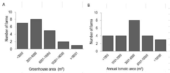
3.1.1 General farm characteristics
The average surface of the farms was 14 ha (range: 1 - 90 ha), however, 78% were smaller than 15 ha. The average surface of greenhouses was 6873 m2, and the planted tomato area was on average 5334 m2 per farm (Figure 1A and B). All farms presented as the main source of income the production of vegetables and the most important product was greenhouse tomato, although some farms had other main crops, such as sweet pepper, lettuce and onion. Productive diversification in the farms varied greatly, from some (two) that were exclusively dedicated to greenhouse tomato, to others that planted more than ten vegetable crops, and nine farms that combined it with animal production: pigs (two), chickens (one) and livestock (six). Most of the farms managed their crops conventionally and two farms had certified organic systems. In terms of commercialization, 83% sold their products through wholesalers in the Mercado Modelo of Montevideo. The rest sold directly to nearby retailers or supermarket chains. Of the total farms, 78% were assisted by technical advisers, mainly focused on greenhouse crops.
Producers were on average 45 years old and had great variability regarding tomato working experience (from three to 22 years). 87% of them integrated local social organizations (development society, cooperative or producer group), and the half actively participated in the activities (more than 3 times per year) of the reference organization. Producers' work during the harvest season (November - April) was on average of 61 hours a week (Range: 48 - 78 h week-1). Once the harvest was over, working hours fell between 20 and 30%. From the total number of producers, 91% were exclusively engaged in farm activity, and only 17% of their spouses worked outside the farm. On average, two family members worked on the farm. The number of hired salaried workers was highly variable, on average two employees were hired per farm, one permanent and one temporary, mainly for harvesting. Organic farms hired more employees permanently and temporarily, especially for product packaging.
All the farms had a tractor to carry out soil tillage and loading tasks. The most widespread spraying tool was the turbine backpack, although the nebulizer, tractor-driven sprayer and common backpack sprayer were also used. The dominant fertigation systems were by venturi (10 farms) and fertilizer tank (eight farms). Only three farms had sorting and/or packaging machinery and a cold chamber. The infrastructure for the classification and packaging of products was very varied, from packing rooms (five farms) to very simple eaves (without walls). 78% of the farms lacked adequate vehicles to transport the products.
3.1.2 Farm groups according to general characteristics and resource availability
The farms were divided into four groups according to the general characteristics and resource availability (Tables 1 and 2). Producers in group 1 had the largest protected area and the lowest proportion of family labor. Organic farms were included. The degree of crop diversification was high and the majority directly commercialized with retailers. The level of mechanization and infrastructure was diverse, but high-level farms were included (Table 1). Group 2 was made up of farms with the least protected area, where most of the workforce was contributed by the family. They were less diverse in terms of production than Group 1 and most of them combined direct sales to retailers with commercialization through wholesalers in Mercado Modelo. Group 3 included farms with a small protected area, where the workforce was mainly family. Commercialization was exclusively through wholesalers in Mercado Modelo. Farms from group 4 had an average protected area of 0.65 ha. Half of the workforce were family members. They presented a low degree of productive diversification compared to the rest of the groups, and sold exclusively through wholesalers.
Table 1: Classification variables for cluster analysis according to group
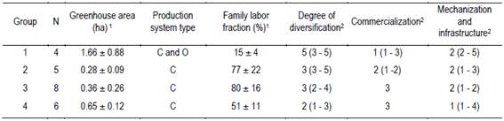
1presents mean ± standard deviation; 2mode is presented (minimum, maximum). N: Number of farms. Production system type: C: conventional; O: organic. Family labor fraction: proportion of the total number of employees. Degree of diversification: 1- tomato only; 2- up to three protected items; 3- up to four protected or field items; 4- more than three protected items and less than three field items, or more than three field items and up to three protected items; 5- more than three field items and more than three in greenhouse. Commercialization: 1- direct sale to retailers; 2- direct sale to retailers and through wholesalers in Mercado Modelo; 3- sale through wholesalers in Mercado Modelo. Mechanization and infrastructure: cold chamber, tomato sorting/packaging, cargo vehicle and venturi fertigation system, or injection pump. They can have 1: none; 2: one; 3: two; 4: three; 5: the four elements.
Table 2: Farm location, main sources of income, wage labor, experience in tomato cultivation, technical assistance and off-farm labor according to the group
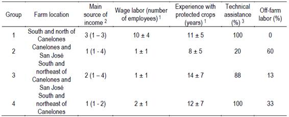
1mean ± standard deviation is presented. 2mode is presented (minimum, maximum). 3percentage of farms with technical assistance in each group are presented. 4percentage of farms where the producer or spouse carries out off-farm labor in each group is presented. Farm location: south (south of route 11), north (north of route 11 and west of route 7), northeast (north of route 11 and east of route 7) of the departments of Canelones and San José. Main source of income: 1- tomato; 2- tomato and sweet pepper; 3- tomato and lettuce; 4- tomato and onion. Wage labor includes permanent and seasonal contracts when they exceed 3 months per year.
Tomato crop was the main source of income in groups 2 and 4, while in group 1, most farms presented tomato and lettuce as the main source of income, and in group 3, tomato and sweet pepper (Table 2). In group 1, farms hired an average of 10 employees, followed by group 4, which hired two employees. In groups 1 and 4, all farms received biweekly or monthly technical assistance, unlike group 2. Group 2 concentrated farms with less experience with protected crops and where off-farm income was frequent.
3.2 Analysis of variability in the economic result of tomato cultivation
A high variability of total and commercial yields and quality was observed among the tomato crops evaluated (Table 3 and Figure 2).
Table 3: Average, minimum and maximum total and commercial yield, large, medium, small and discard category fractions
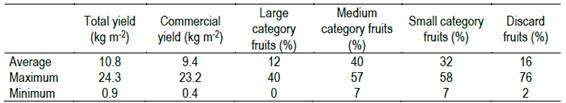
Fruit categories according to size: large (> 80 mm), medium (65-80 mm), small (50-64.9 mm), and discard (<50 mm).

Tomato wholesale prices were very dynamic throughout the year (Figure 3). The average wholesale price for the medium-sized tomato (65 - 80 mm) was 43.5 $U (range: 12 - 87 $U kg-1) and 43.7 (range: 24 - 80 $U kg-1) per kilo in 2014/2015 and 2015/2016, respectively. However, during the greatest tomato supply period in the south of the country (November to May), the average price was 41.1 $U kg-1 in 2014/2015, higher than 29.9 $U kg-1 in 2015/2016. Prices were higher from January to April in 2014/2015, and for several weeks of June, September and October in 2015/2016. The lowest prices, in the greatest supply period in the south, in the year 2015/2016 coincide with a higher production of the evaluated crops compared to the previous year (Figure 4). Large Category prices (>80 mm) were on average 32.4 and 48.8 $U kg-1, and 16.8 and 33.6 $U kg-1 for the small category (50 - 64.9 mm) in 2014/2015 and 2015/2016, respectively.
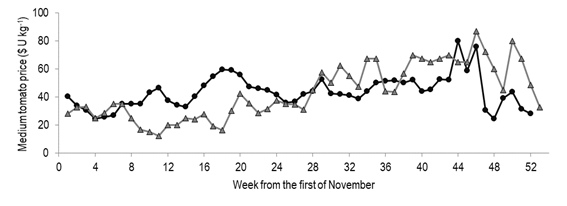
Figure 3: Weekly evolution of the wholesale price of medium category tomato (65-80 mm) in the Mercado Modelo of Montevideo in 2014/2015 (●) (11/1/2014 - 10/31/2015) and 2015/2016 (▲) (11/1/2015 - 10/31/2016)
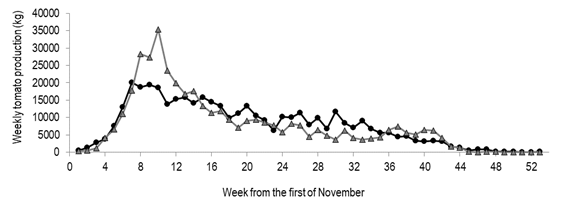
Figure 4: Weekly evolution of commercial tomato production in the greenhouses under study in the years 2014/2015 (●) (11/1/2014 - 10/31/2015) and 2015/2016 (▲) (11/1/2015 - 10/31/2016)
Significant variability in costs was found among the evaluated crops (Table 4). The main component within production costs was due to labor cost. Followed by commercialization costs (transport and commission) and greenhouse devaluation. Inputs with the greatest associated costs were seeds, young seedlings, and fertilizers. Input cost was positively correlated with the total yield (Spearman Correlation Coefficient - 0.52; p-value <0.0001). Yields greater than 20 kg m-2 were only obtained with input costs above 1 usd m-2, however, above 1.3 usd m-2 no yield increase was observed (Figure 5). Each input cost level showed great yield variability. Some producers achieved yields of 10.4 kg m-2 with minimum cost, while others did not exceed 1 kg m-2.
Table 4: Average, maximum and minimum of total costs, labor, commercialization, greenhouse devaluation, seeds and plants, fertilizers, phytosanitary products, irrigation, mulch and conduction inputs costs
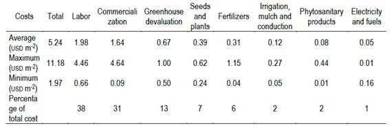
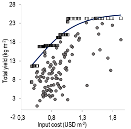
Figure 5: Total observed yield (●), boundary points (□), and boundary line function according to input costs
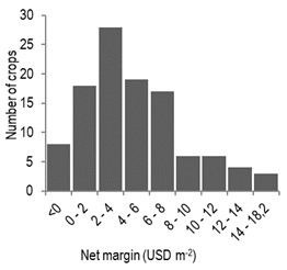
The variability found in yields, prices, and production costs lead to differences in gross income and net margins by area (Figure 6). The average net margin was 4.82 usd m-2 (range: -1.37 - 16.21 usd m-2). Gross income was between 0.70 - 24.51 usd m-2 with an average value of 10.05 usd m-2.
The variability found in the net margin can be attributed primarily to the differences in gross income (Figure 7). The crops with the highest gross income (>=11.8 usd m-2) had an average net margin of 9.38 usd m-2, while those with lower gross income obtained an average net margin of 2.75 usd m-2. Within the low gross income group, crops with higher commercial yields obtained higher average net margins. Within the highest commercial yield group, those with less than 24.6% of small fruits scored higher net margins. Within the group with the highest proportion of small fruits, the average price per kilo explained the differences in net margin. Within the group with sales price lower than 1 usd kg-1 the differences between crops were explained by differences in commercial yield. Low gross income crops (<11.8 usd m-2) and low commercial yield (<4.53 kg m-2) were partitioned according to the medium size fruit fraction. Within the high gross income group (>=11.8 usd m-2), crops with higher selling price obtained higher net margins. And within this group, the differences in the net margin were attributed to differences in the amount of medium-sized fruit. Among those who received an average price lower than 1.11 usd kg-1, those that spent more than 0.39 usd kg-1 had a lower average net margin. The characteristics of the identified terminal groups (tg) are presented in Table 5.
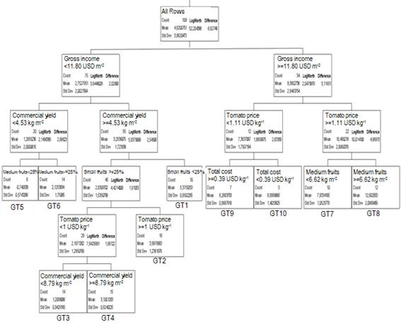
Table 5: Characteristics of the resulting groups of the regression tree

TG: Terminal group N: Number of cases. 1presents mean ± standard deviation; 2presents the percentage of farm groups 1, 2, 3, and 4 respectively. Input output ratio: Ratio of total costs to gross income
Each box corresponds to the group data, the initial box (all rows) corresponds to the total of crops analyzed, the terminal groups (TG) result from the successive binary partitions. Each partition is associated with a variable and a threshold value in the unit of the variable that divides the largest group into two subgroups. Each bold box shows the variable and the threshold that generates the partition and identification of that subgroup, the statistical significance of the partition by this variable is shown in the next box above as LogWorth, where LogWorth = -log10*(p-value). Each group is described by the number of crops it covers (count), the average value of the dependent variable for the group (mean), and its standard deviation (Std Dev). In this case, 10 TG were formed, N = 109, number of partitions = 9, R2 = 0.900.
Each box corresponds to the group data, the initial box (all rows) corresponds to the total of crops analyzed, the terminal groups (tg) result from the successive binary partitions. Each partition is associated with a variable and a threshold value in the unit of the variable that divides the largest group into two subgroups. Each bold box shows the variable and the threshold that generates the partition and identification of that subgroup, the statistical significance of the partition by this variable is shown in the next box above as LogWorth, where LogWorth = -log10*(p-value). Each group is described by the number of crops it covers (count), the average value of the dependent variable for the group (mean), and its standard deviation (Std Dev). In this case, 10 tg were formed, N = 109, number of partitions = 9, R2 = 0.9. The group defined based on the general characteristics and available resources on the farms was not among the main causes that explained the variability in economic efficiency. The different groups are present at multiple levels of economic and labor efficiency (Table 5). In this way, producers from groups 1 and 2 are present in both the terminal group with the highest average net margin (terminal group 8), and the negative average net margin (terminal group 5). However, groups 1 and 4 presented higher averages than groups 2 and 3 in commercial yield, gross income, total cost, net margin, and labor efficiency (measured as net income and commercial production per hour worked) (Table 6).
Table 6: Commercial yield, total cost, gross income, net margin, and labor efficiency according to the group to which the farm belonged
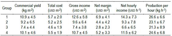
Mean ± standard deviation is presented.
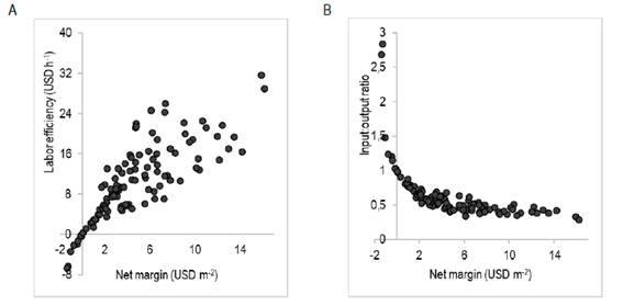
A very important variation was observed in the net income per hour worked for net margins greater than 2 usd m-2; for example, for the net margin level of 6 usd m-2, crops with a net income per hour worked between 6 and 24 usd h-1 were observed, which is equivalent to labor requirements of 1 and 0.25 h m-2, respectively (Figure 8A). The Input:output ratio was kept at levels between 0.4 and 0.6 when the net margin varied from 3 to 14 usd m-2, but increased significantly to net margin values lower than 3 usd m-2 (Figure 8B).
4. Discussion
4.1 Characteristics of farming systems
Four groups of farms were distinguished according to general characteristics and resource availability. Knowing the differences between tomato farms in the south of the country is valuable to design innovative systems according to the structural and functional possibilities of each farm. Group 1 consisted of larger-scale farms with a high requirement for wage labor. This group of producers, unlike the rest, does not qualify within the current definition of family farmer determined by the Ministry of Livestock, Agriculture and Fisheries, since they hire more than 5 employees permanently or their equivalent in temporary employees1. Group 2 included farms with smaller protected areas and a mostly family workforce, with a moderate to high degree of product diversification and commercialization through different channels. This type of family farms with limited area uses productive diversification as a tool to face risks in the best way and ensure livelihoods18)(19. It is the only group in which off-farm work of the producer or spouse predominates. In most cases, the wives are the ones who work outside the farm and contribute a fixed salary to the family income. Off-farm labor is also considered a way to diversify income to minimize the risks of productive activity and is fostered by: greater risk aversion, high variability in farm income, less experience in productive activity, and a smaller scale20. Commercialization ways of groups 3 and 4, exclusively in Mercado Modelo through shippers and wholesalers, are related, among other factors, to the fact that most farms do not have cargo transportation for the products (low mechanization and infrastructure index). This makes them dependent on intermediary’s services. The cost of these services represents on average 31% of the total production costs, being one of the main costs. The producers who depend on other agents to access the market are the weakest figures in the horticultural chain. They have no negotiation power because of the lack of necessary transportation, but also their production scale does not allow them to take their produce to the market in a profitable way21. This separates them from the clients, restraining direct information on operations, quality, and prices.
It should be noted that this farm classification does not represent the totality of farms in the area and is limited to the variability collected in the sample. The sample size (10% of the study population) was limited compared to the recommended (50 farms) for statistical reasons22 for this type of study. This can affect the proportion of farms belonging to each group and, if there is a small group represented by one case in the sample, it would be considered atypical or combined in another group in the multivariate process23.
4.2 Main factors affecting net profits in tomato cultivation
High variability was found in commercial yields, qualities according to size, sale prices according to the harvest season, and production costs. This resulted in net margins ranging from negative values up to a maximum of 16.2 usd m-2. The main cause of these differences in seasons 2014/2015 and 2015/2016 was the variability of gross income by area. Productivity (yield and quality) and price explain the net margin differences for all gross income levels. However, the price is more relevant in the group with the highest gross income, and yield in the group with the lowest gross income. Production costs were only ranked for crops with the highest gross income. These results demonstrate that the improvement of the family income, through the improvement of the net margins of the crops, will have to consider different strategies according to the starting gross income level. If it is low, it should be aimed at improving yields and quality; on the other hand, if it is high, it should work on reducing costs, improving prices or increasing yields for the fruit's categories of higher sale prices. In most of the crops analyzed (82%), the gross income was low (<11.8 usd m-2), so improving the yields per area is essential to improve economic efficiency in most cases. There is great variability in yields between tomato crops and farms in southern Uruguay, and a gap relative to attainable yield (maximum yield obtained in the area) estimated at 5.2 kg m-2(10. This variability and the gap are mainly explained by differences in crop management (transplant date, cycle length, greenhouse transmissivity, defoliation intensity, potassium management, irrigation, among others)10. These differences in management practices are mostly associated with knowledge gaps between producers10, and not with differences in resources availability (social and economic capital) in farming systems that limit management intensification and, consequently, productivity, as mentioned by other authors16. The farm group variable defined according to general characteristics and resources available on the farms was not ranked among the main causes of variability in the economic efficiency of tomato cultivation. Farms with different production scale, infrastructure and resource endowment reached high net margins in tomato cultivation. This situation differs from numerous studies that highlight the significant impact of the structural characteristics and resource availability of farms on productivity, economic efficiency and labor efficiency5)(8)(9)(24)(25)(26. Despite the minor importance of the farm group in the definition of the economic efficiency of tomato cultivation, farm groups 1 and 4, that presented the largest protected area and the largest proportion of wage labor, obtained, on average, higher: yields, total costs, gross income, net margins and labor efficiency in tomato cultivation. Farm group 1, with the largest scale and the greatest development in the commercial area, prevailed in the terminal groups with the highest average net margin (tg 7, 8 and 10). On the contrary, farm groups 2 and 3, with a smaller scale and less resource availability, prevailed in terminal groups with lower average net margin (tg 3, 5 and 6). Farm group 1, which included organic farms, obtained the highest average yield and economic efficiency. This contradicts other studies reporting lower yields in organic systems compared to conventional systems15)(27)(28. It should be clarified that the organic systems in the sample were only two and probably do not represent the great variability present in the organic systems in the study region.
Prices are not controlled by producers, but there might be room for improvement by exploring different commercial alternatives and increasing the fruit fraction of the categories with the highest selling price. High price variability was observed throughout the year, associated with differences in supply and demand, so different harvest times generate important differences in prices. The other relevant factor is the quality of the harvested product. Medium tomato has a higher price than the other categories. On average, large and small categories had prices 7 and 42% lower than the medium, respectively. Moreover, the price could differ due to the presence of defects (cracks, yellow shoulders, insect damage and diseases), which was not taken into account in the analysis. Prices for a tomato quality at any given time may vary according to clients and commercial strategy. This source of variation, and how it affects profit margins, was not analyzed in this study, because Mercado Modelo prices were used for all crops.
The main production costs were labor (38%) and commercialization (31%), while inputs represented 15%. Given that commercialization expenses depend on third parties who provide these services, the alternative to reduce costs at farm level lies in improving the efficiency of the use of inputs and labor. A positive correlation was observed between input costs and total yield. This may be due to the fact that long tomato cycles of more than 200 days have higher yields than short cycles, and, in turn, require more inputs such as fertilizers and pesticides10. In any case, an important variability in the obtained yield was observed for each level of input cost, which can be associated with different crop management with the same input set, resulting in differences in the efficiency of their use. The crops with the highest net margin were the most efficient in the use of inputs and labor. However, labor efficiency varied significantly when the net margin exceeded 2 usd m-2. This indicates that for the same net margin there were different intensities of work (hours per surface), that resulted in different efficiencies. The working hours depend on the management of each crop (plant lowering, pruning, leaf removal and harvests), and equipment availability, such as fruit sorting machine for the preparation of the product for sale and hand-operated sprayers or fixed nozzles for the application of agrochemicals. These tools can significantly reduce labor needs.

