


Servicios Personalizados
Revista

Articulo
 Inglés (pdf)
 Articulo en XML
 Referencias del artículo
Links relacionados
Compartir

 Permalink
CLEI Electronic Journal
versión On-line ISSN 0717-5000
CLEIej vol.19 no.1 Montevideo abr. 2016
An Adaptive and Hybrid Approach to Revisiting the Visibility Pipeline
Abstract
We revisit the visibility problem, which is traditionally known in Computer Graphics and Vision fields as the process of computing a (potentially) visible set of primitives in the computational model of a scene. We propose a hybrid solution that uses a dry structure (in the sense of data reduction), a triangulation of the type  , to accelerate the task of searching for visible primitives. We came up with a solution that is useful for real-time, on-line, interactive applications as 3D visualization. In such applications the main goal is to load the minimum amount of primitives from the scene during the rendering stage, as possible. For this purpose, our algorithm executes the culling by using a hybrid paradigm based on viewing-frustum, back-face culling and occlusion models. Results have shown substantial improvement over these traditional approaches if applied separately. This novel approach can be used in devices with no dedicated processors or with low processing power, as cell phones or embedded displays, or to visualize data through the Internet, as in virtual museums applications.
Abstract in Portuguese:
Revisitamos o problema de visibilidade, que é tradicionalmente conhecido nas áreas de Computação Gráfica e Visão Computacional como o processo de computar um conjunto de primitivas de uma cena (potencialmente) visíveis. Propomos uma solução híbrida que usa uma estrutura enxuta (no sentido de redução de dados), uma triangulação do tipo J1a, para acelerar a tarefa de procura por primitivas visíveis. Chegamos a uma solução que é útil para aplicações interativas, on-line, e de tempo real, tal como visualização 3D. Em tais aplicações, o objetivo principal é carregar uma quantidade tão mínima quanto possível de primitivas da cena, durante o estágio de renderização. Para este propósito, nosso algoritmo executa o recorte de primitivas usando um paradigma híbrido baseado nos modelos ”viewing-frustum”, ”back-face culling” e ”occlusion”. Os resultados evidenciam melhoras substanciais sobre esses modelos, se aplicados separadamente. Este novo método pode ser usado em dispositivos sem pro cessador dedicado ou com pouco poder de processamento, como telefones celulares ou dispositivos de visualização embarcados, ou também para visualizar dados pela Internet, como em aplicações de museus virtuais.
Keywords: Visibility; Visualization Structure; Real-time 3D Visualization; Hidden Primitive Culling.
Keywords in Portuguese: Visibilidade; Estrutura de Visualização; Visualização 3D em Tempo-Real; Recorte de Primitivas Escondidas.
Received: 2015-11-10 Revised: 2016-04-04 Accepted: 2016-04-11
DOI: http://dx.doi.org/10.19153/cleiej.19.1.8
1 Introduction
We revisit the solutions for the visibility problem, which is the process of computing a potentially visible set of primitives in a scene model, intended for interactive and real-time applications. We came up with enhancements in the visualization pipeline by using a visualization structure that minimizes the amount of useless data being loaded to generate the visualization of a given scene. Basically, we accomplish this by dividing the scene into a special grid, upon the  structure (a triangulation), then associating to each grid block the primitive(s) that belong to it and finally determining the visible set of primitives. On the way of visibility determination, several primitives and blocks are automatically hidden by others, thus without need of testing these in the visibility processing pipeline. As a novelty, our method makes use of the
  triangulation structure [1] to create the subdivision grid. We have chosen this structure due to its algebraic (easy of computing and store) and adaptive (can be used with irregular data) useful features.
1.1 Visibility culling
In 3D graphics, hidden surface determination, which is also known as hidden surface removal, occlusion culling or determining the visible surfaces, is the process used to compute which parts of the surfaces are visible and, consequently, which ones are not visible from a certain point of view. An algorithm for hidden surface determination is a solution to the problem of visibility, which is known to be the one of the first major bottlenecks in the area of 3D computer graphics [2]. The process of hidden surface determination is sometimes called hiding. The analog problem for lines is to render the hidden line removal. Determining the hidden surfaces is required to process the scene and produce an image properly, so that one cannot look through (or walk into) the walls in virtual reality applications, for example.
Besides the advances in hardware technology and software experimented in the last decades, the visibility determination has yet being one of the main issues in computer graphics and vision. Several algorithms capable of removing hidden surfaces have been developed to solve this problem [2]. Basically, these algorithms determine which set of primitives that make up a particular scene are visible from a given viewing position. In fact, Cohen et al. [2] argue that the basic problem is mostly solved, however, it is known that, due to the constant demand for higher amount of 3D data, mainly in massive data applications, algorithms such as Z-buffer and other classical approaches may have trouble while trying to guaranteeing the visualization of the scene in real-time. The computation of the visible surfaces may be impractical depending on the system demand and resources available. Of course, agreeing to Cohen, one can find works in the literature such as Jones [3], Clark [4] and Meagher [5] that addressed this issue in the very beginning of CG. Nonetheless, we recall the attention to the actual importance of this problem during evolution of CG. Even latter, researchers as Airey et al. [6], Teller and Sèquin [7, 8], and Greene et al. [9], focused their work on this issue and have studied the problem of visibility trying to speed up visualization.
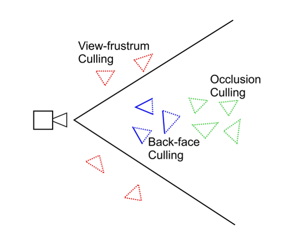
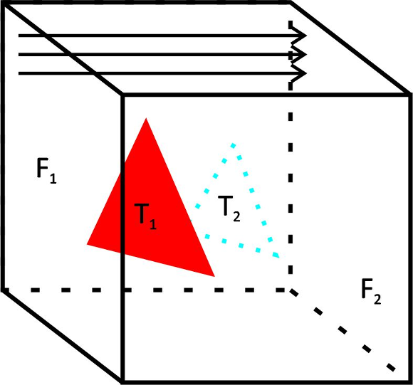
To better understand the pipeline, the process starts with visibility culling that aims to quickly reject primitives that do not contribute to the generation of the final image of the scene. This step is done before the step of hidden surface removal is performed, and only the set of primitives that contribute at least to one pixel in the screen is rendered. Visibility culling is executed using the two following strategies: back-facing and viewing-frustum culling [10]. Back-face culling intends only to use primitives looking at (facing to) the camera display (the viewing plane), and view-frustum culling rejects primitive located outside the visualization frustum, which is intended to be the only visible portion of the scene. Over the years, efficient hierarchical techniques have been developed [4, 11, 12], as well as other optimizations [13, 14] in order to accelerate visibility culling. Besides these previous techniques, the occlusion culling process avoids rendering primitives that are hidden (occluded) by other primitives in the scene. This technique is more complex because it involves an analysis of the overall relationship between all primitives in the scene. Figure 1 illustrates the relation between the three known culling techniques.
Since these traditional contributions studying the visibility culling, as cited above, and some few further contributions [15, 16, 17, 18], not recent, which will be better explored in Section 2, we could not find any up to date literature on this subject. As there are currently many on-line and real-time 3D world navigation applications (as virtual museums or buildings visualization) that require significant amount of primitives to be rendered in real-time, we have been motivated to revisit the visibility problem to see whether it can not be even enhanced. In fact, we observe that the above techniques have some difficulties as the complexity of the occlusion culling to analyze the whole scene or the amount of computations in order to determine primitives facing sides (vector products) or if primitives are inside the frustum in the visibility culling methods. These are not trivial mainly in massive data applications or where the scene is modeled at once for example. This may occur in several applications as in a museum scene where there are too many sculptures, for example, or in outlooking scenarios such as a city landscape.
1.2 Contributions
We overcome the above mentioned difficulties by proposing a different approach introducing and adapting the above simple techniques to our context. We employ a visualization (spatial) data structure that is capable of fast obtaining a potentially visible set of primitives of the scene from the viewpoint of a user. As said above, this structure is constructed by subdividing the whole scene into a grid based on a triangulation of the type  . With this, we achieve significant improvements on the results, as it will be shown. In particular, our method can handle this kind of data reducing the resources requirements. In the experiments, we verify a removal gain of 15% to 20% of primitives for single objects and could observe several other interesting results that validate and also delimit our approach. These will be better discussed during the paper and mainly in the experiments and results section.
So the main contribution of this work is the in the visualization pipeline itself, which is based on a hybrid approach upon an adaptive structure that is capable of determining occlusion culling in two ways: internal block occlusion and adjacent block occlusion. The use of algebraic functions for fast access of block culling, block faces and adjacency is also another contribution that has helped enhancing the visualization process.
Another contribution of using this structure is that it can also be used to determine a hierarchical order of graphics data transmission often necessary in on-line applications. In case of a Virtual Museum application, for example, it can be used to determine the visible set of primitives at the starting point of simulation. So in this case our structure can be used not only to minimize the amount of data in the visualization phase but also in the transmission phase of on-line applications.
2 Related work
Since viewing frustum and back-facing culling are mostly trivial to determine, the recent literature up to this point has mostly focused on occlusion culling. One of the most valuable works that we found in this subject area is the one of Cohen et al. [2] that is also a very useful survey. They subdivide and classify the various occlusion culling techniques developed proposing a classification of the various methods in accordance to their characteristics, as seen in the next subsections.
2.1 Techniques classification
The occlusion culling methods can be classified as point based or region based methods. Point based methods execute their computations from the perspective of the camera view point. On the other hand, region based methods perform their computations from a global point of view that is valid from any region of the scene. Point based methods can be classified as:
- Image Precision Methods - generally operate with the discrete representation of the objects when they are broken into fragments during the rasterization process. Among these are the Ray Tracing [19, 20, 21, 22, 23] and the Z-buffer [9, 24, 5, 25, 26] based methods that are the most common.
- Object Precision - use the raw objects for the computation of visibility. Among these methods we can find the works done by Luebke and Georges [27] and by Jones [3].
On their turn, the region based methods can be classified as:
- Cell-and-Portal - Starts with an empty set of visible primitives and adds them through a series of portals. Among cell-and-portal based methods we cite works by [6], [8].
- Generic Scenes - Initially assumes that all primitives are visible and then eliminates if they are found to be hidden.
Cohen et al. [2] also devised several other classification criteria. For that, some dichotomies were established by Cohen et al. [2]. One of these is looking if a method overestimates the visible set (conservative) or if it approximates it, and what is the degree of over-estimation for the conservative methods. Other is if a method treats the occlusion caused by all objects in the scene or just of a selected subset of occluders. Also, looking if each occluder is treated individually or as group to be more precise. If the method is restricted to 2D floor plan or can they handle 3D scenes. Other simple criteria are: if the method executes a precomputation stage; if it requires special hardware in order to perform the precomputation stage or even the rendering stage; and, finally, if it can deal with dynamic scenes.
2.2 Recent approaches for visibility
Bittner et al. [15] propose a from-region visibility method where rays are cast to sample visibility. The information from each ray is used for determination of all viewing cells that it intersects. They use adaptive sampling strategies based on ray mutations that exploit the coherence of visibility. Chandak et al. [16] propose a method that has some similarity to ours. Their approach uses a set of high number of frusta and computes blockers for each one using simple intersection tests. They use this method to accurately compute the reflection paths from a point sound source. The method proposed by Tian et al. [17] integrates adaptive sampling-based simplification, visibility culling, out-of-core data management and level-of-detail. During the preprocessing phase the objects are subdivided and a bounding volume clustering hierarchy is built. They make use of the Adaptive Voxels, which is proposed as a novel adaptive sampling method applied to generate level of detail models. Antani et. al. [18] introduce a fast occluder selection algorithm that combines small, connected triangles to form large occluders and perform conservative computations at object-space precision. The approach is applied to computation of sound propagation, improving the performance of edge diffraction algorithms from a factor of 2 to 4. Carvalho et al. [28] proposed an improvement to the visualization frustum culling method by using an octree based space partitioning method. This method is in some way similar to ours. The basic difference is that while their method partitions the view frustum, in our method the visualization frustum uses preprocessed data from our space partitioning structure.
2.3 Contextualization
Our method is classified as a region based method, somewhat similarly to the cell-and-portal. The main differences with that are that instead of a set of cells we use the scene subdivision grid, and that instead of a portal we use the adjacency between grid blocks. This has proven experimentally to be useful as well, at least.
Following the other cited criteria of Cohen et al. [2], our method overestimates the potentially visible set. We discuss the degree of over-estimation in Section 5.1. Though occlusion detection is block based, our method treats the occlusion created by all the blocks in groups. Our method handles 3D scenes and, due to the  triangulation structure, we believe we can add a fourth dimension for animation applications.
Our precomputation stage executes without the need of a special hardware, though the use of a dedicated graphics processor would even speed-up the processing. We intend to implement this feature later on and also take advantage of parallel processing to speed up the internal and adjacent block culling stages.
So far we treat dynamic scenes (with moving objects) by ignoring the occlusion made by the moving objects. This means that if a moving object inside the viewing frustum passes in front of other objects (or primitives), these are also precomputed as visible, thus not influencing the final visualization of the occluded objects. Of course, the final visualization will have to deal with these extra primitives given by the procedure (and it will) by computing which one is truly visible (the object or the occluded primitives). We consider that this overestimation is better than trying to determining from a frame to another where the moving object is and then recomputing the whole grid at once. Of course, this could be understood as a drawback of our method if we consider that most of the objects of a scene is moving, on the worst case. However, nonetheless, we do not know any method that treats this, the applications the method is devised for (museum applications and sending 3D data through Internet) have not that huge amount of moving objects in their environments. Because of this we do not show results based on moving objects. Besides, results for the camera moving are shown.
3 Solving visibility with the  triangulation
We base our visualization scheme on the algebraic features of the  using it basically as a spatial data structure. The whole 3D scene is initially contained within the grid created by the initial
  structure. A initial step is performed in which the primitives of the model are related to (pointed from) each element of the spatial data structure in such way that is contains information of what are the visible set of elements in a given positioning of the camera. From the point of view of the camera, the idea is to traverse the
  structure calculating all visible elements in it. So every time that the camera moves the calculation of the visible set of primitives is redone traversing the
  structure.
The  triangulation [1] is an algebraically defined structure that can be built in any size. To accommodate local aspects, the
  triangulation handles refinements naturally. Two of its main characteristics are the existence of a mechanism to uniquely represent each simplex of the triangulation and the existence of algebraic rules to traverse the structure. Using these rules prevents the structure need of storing connectivity information of simplices thus enabling more efficient storage.
Formalizing, the  triangulation consists of a computational grid formed by n-dimensional hypercubes (blocks). Each block is divided by
  n-simplices that can be described algebraically using the sixfold:
The first two elements of  defined in a block are contained in the simplex, being a vector
  with
with  -dimensional coordinates indicating that the block is in a particular level of refinement
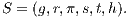
  in the grid. Figure 2, left, illustrates a two-dimensional grid of
  and, right, a block of this outstanding level of refinement grid with
  (0-block) and
  . Also in Figure 2 it can be noticed that the blocks are darker for grid level r = 1 (so is called 1-block) and hence that they form part of a region of the grid of higher resolution.
 (left) and details of the block
  ,
,  where it is shown two paths for tracing the block simplices.
Since the  triangulation is naturally adaptive, this helps in making this structure more precise when it comes to over-estimating the potentially visible set from the scene. This is because, with more refined (smaller) blocks in certain regions of the scene, more blocks are fully filled. Due to this, the adjacent block occlusion culling can be more common and thus more effective.
Since we are using  triangulation structure in this work for a purpose other than triangulating, from now on we will refer to its basic grid as the
  structure.
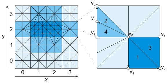
4 Technique overview
Figure 3 illustrates the overview of our technique. Basically, it is subdivided into two stages: the preprocessing and the visualization (visibility precomputation) stages. In the following we better detail these stages.
 grid, after which the visibility precomputation stage is executed to generate the primitive list for each the point of view on the grid blocks.
4.1 Preprocessing stage
During the preprocessing, we use the  structure basic grid to generate the visualization blocks. The preprocessing stage is done in three steps:
- Given the user input where it is established the minimal dimension of the grid along one of its axis, we determine the size of the grid’s edges and then calculate the rest of the grid’s dimension.
- Each triangle is firstly mapped to the grid block(s) where it is contained;
- By using the triangle’s normals we identify what face of the block(s) the triangle is looking at. In this step we automatically treat the back-face culling (this is calculated once even if the camera moves);
Internal block occlusion can then be calculated using an approach similar to Z-buffer. The final list of primitives is assigned to each block faces. During this step we can find out if the block face is fully filled, this is needed to determine adjacent block occlusion in the visualization stage. This step is illustrated in Figure 4.
4.2 Visibility precomputation
We use the grid to verify what elements are being directly looked at. Given the camera position ( as illustrated in Figure 5) and its look-at vector, we use the
  structure transition function to access the blocks in its line of sight. The look-at vector is also used to determine which block face(s) will be used to compose the final list with the potentially visible set of primitives. Our visualization structure determines occlusion culling in two ways: internal block occlusion and adjacent block occlusion.
4.2.1 Internal block culling
Internal block culling occlusion is identified using only the primitives inside each block and it is done for every block face as illustrated in Figure 4 for face  . This approach is similar to the Z-buffer technique storing the depth for each ray that is cast for a given grid face. When verifying the visible set of triangles for a given face
  , if the rays determine that a triangle
  completely hides a triangle
  so this last is not pointed as visible for face
  .
.
 , the rays determine that triangle
  hides triangle
  .
.
4.2.2 Adjacent (external) block occlusion
Before each transition from block to block the visible face of the current block is verified in order to determine if it is fully filled, this is to permit the operation. If the case is true, fully filled, this means that the visible set from that face totally hides the visible set from its adjacent block face, so the hidden block and its subsequent adjacent blocks are not needed for the rendering stage. The transition step for adjacent block occlusion determination is illustrated in Figure 5. Note in the Figure that after visiting the block  the blocks
  ,
,  and
and  are queued to be visited next. After visiting block
  and determining that its visible face is fully filled, the next adjacent blocks are not directly added to the visitation cue. But there might be a case, in this example, where the block
  adds one or more of these adjacent blocks to the cue.
Note that at the end of this second phase blocks occluding other blocks are determined thus complementing the internal block occlusion process.
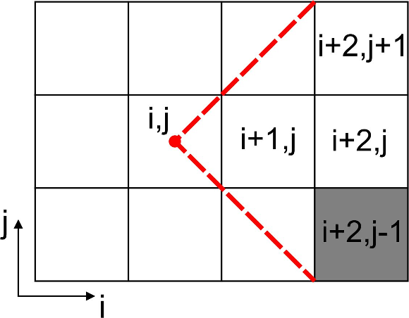
 is fully filled, so the next adjacent blocks are not directly added to the visitation queue due to it (they might be added due to another block).
4.3 Visualization (rendering)
Finally, once the  data structure contains pointers to the visible set of primitives, the step for computation of the visible set of primitives for rendering of the data can then be executed. To do so, the list of (visible) blocks faces is visited and used to compose the potentially visible set. We remark that at least the visible set is pointed by the grid data structure, from which the rendering stage can then visualize the really visible ones. As shown in the results, this overestimation rate is low thus allowing a fast processing of the data in the visualization process. As previously said, every time the camera is moved to another block or its look-at vector is changed, the calculation to obtain the visible set of primitives has to redone.
Also, the  structure is capable of dealing well with primitive transparency in the case of both types of occlusion culling. It does so during the internal block occlusion phase. When the ray encounters a transparent/semi-transparent primitive, that primitive is tagged for transparency processing and the ray will continue to try and find another primitive along its path. In this way, transparency can be calculated from primitive to primitive composing the final value of intensity for a given ray.
5 Experiments and results
To assess the efficiency of our visualization structure, we have planned and performed a series of experiments. We executed experiments where each visibility model is visualized individually, experiments where the camera is statically positioned, and experiments where the camera navigates along the scene.
It is worth mentioning that our experiment does assess loading time since this stage is precomputing stage. Our main goal here is to assess real-time visualization efficiency. This does not mean that loading performance will be ignored, in later stages of this work we intend to implement the parallelism paradigm in stages such as the internal and adjacent block culling stages.
5.1 Experimental setup
The first series of experiments are devoted to assess the visualization structure’s efficiency. These experiments were done on an Intel Core i7 2.00GHz PC with 8GB Ram, with a Radeon HD 6770Ms Graphics Card and running on Windows 7 (64bits).
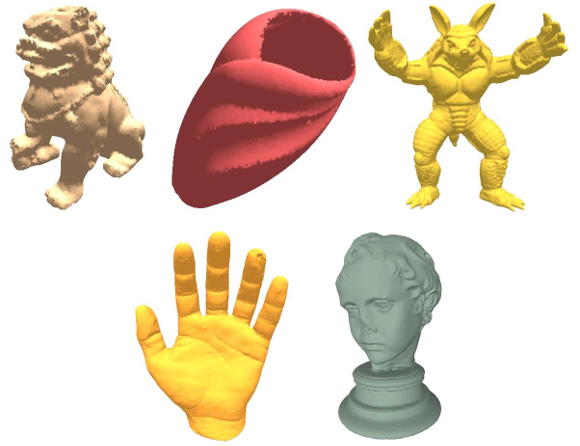
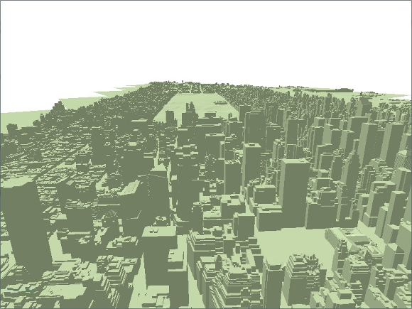
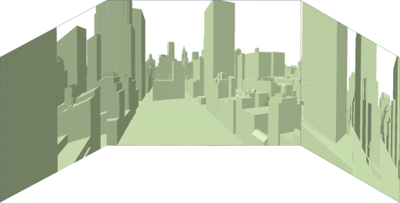
For these experiments, we use a series of simple mesh models obtained from the Aim-at-Shapes Repository: Chinese Lion (identified as i in result tables), Vase (identified as ii), Armadillo (identified as iii), Hand (identified as iv) and Eros (identified as v), and also use the Manhattan model (identified as vi). This model was developed by Andrew Lock and is available for purchase at the 3D Cad Browser homepage (available at http://www.3dcadbrowser.com), being composed by a set of 306 meshes with a total of 3.6 million polygons, 5 million vertices and 296 texture images each one with the resolution of 4096x4096. This model is a great study case as it has all primitives forming a unique model of the scene. Figures 6 and 7 illustrate each model. The models’ shape characteristics and high level of detail makes them ideal to test our structures’ efficiency for visualizing individual meshes.
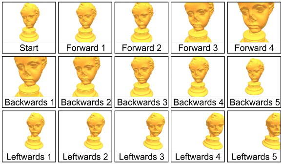
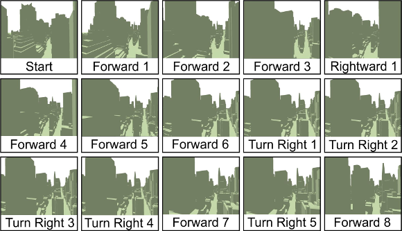
Figures 8 and 9 illustrates the series of navigation steps taken during the experiments. For the simple meshes we use the steps in Figure 8 and for the Manhattan model we use the steps illustrates in Figure 9.
5.2 Evaluating resulting data
During the experiments, we basically verify the following resulting data:
- The mean frame rate (still (A) and navigation (B)) in comparison with using the whole data, without our technique (C). This kind of metric is a basic measure for any interactive 3D application and is generally measured in frames per second.
- Mean ratio (B) between the potentially visible set and the total number of primitives of the scene (#Pri). We also analyze the mean ratio of only using view-frustum and back-face culling (A) with the #Pri, we verify this to identify the proportion of elimination from each culling technique. The values range is
 and can be interpreted as for example: if ratio is equal to
  then this means that the method eliminates
  of the original primitives.
 - Mean overestimation ratio as proposed by Cohen et. al. [2], where we compare the ratio between the size of the visible set (VS) and the size of the potentially visible set (PVS), in other words the ratio is equal to
 .
.
Just like the first result data set, we calculate the mean value of the data in the second and third data set after each scene navigation. For each result data set we also present its standard deviation ( ). In order for providing a fair comparison between each ratio value, the same sequence of the scene navigation steps are made for every experiment executed in each model.
Tables 1 and 2 present the resulting data detailed above obtained during our experiments. As we mentioned previously, the experiments executed in each model are done using the same sequence of navigation steps and same grid dimension.
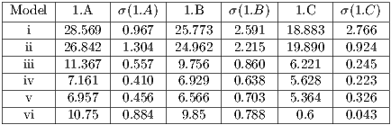
As we can see from Table 1 the frame rate obtained when visualizing each model using the visualization structure is better than using the whole data of the model. This result only ascertains that the structure is working properly, the important results from this series of experiments is if the recalculation of the visible set affects the frame rate. By comparing columns 1.A and 1.B we can see that the recalculation step executed along the navigation sequence does not affect the frame rate too much, lowering it at most by  .
.
 (
( ) and the mean rate (and standard deviation) of PVS in relation to
  (
( ). We also analyze the rate between the number of primitives that are really visible and the size of the potentially visible set of primitives for experiment (
 ).
).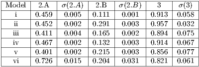
In Table 2, we can see that the reduction of data being used for the visualizations stage is quite significant. Although the back-face culling did most of the hidden primitive removal, the occlusion culling still removes a reasonable amount of hidden primitives. And in the case of the vase, due to its concave shape, we can see that the occlusion culling removes a higher proportion of primitives. It removes  in comparison to the other models where a rate lower than
  is removed.
From these results, we can figure out that, since the models that we use in each experiment are single object meshes, the occlusion culling does not remove as much primitives because of the actual lack of occlusion that occurs in the respective scene. In the same manner, the overestimation ratio is low due to the use of the single object meshes. At most the possible visible set is higher than the visible set by  .
.
When we analyze the overestimation ratio of our method in comparison with previous works, we could find out that the visible set has a roughly similar ratio, ranging from  For the three biggest models used during the experiments, the preprocessing stage took
  seconds to execute. Though we are showing this as a result of the visualization structure, the execution of this stage does not affect the visualization stage itself. And, in many cases, once the precomputation stage has been executed, the program application can just store the data obtained.
5.3 Visual quality assessment
Besides the importance of testing the efficiency of the structure parameters, it is also important to assess the visual quality of the graphic objects and scenes. In this case, we want not only to visually verify the existence of possible missing primitives (holes) but also to use the same ray-tracing based algorithm to determine if any ray cast from the point of view does not intercept a primitive where it should not have done so. So far we performed extensive visualizations over the data to verify that, and this has not been the case in our tests.
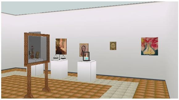
Another quality test that we executed is the application of our structure in a Virtual Cave for visualizing different points of views. As illustrated in Figure 10, we simulated this scenario by composing our scene using three projection planes on the scene. In this case, we once again not only tested the structures efficiency in regards to individually determining the visible primitive set for each point of view but also assessed its visual quality.
6 Conclusion
We introduce a new visibility paradigm based on the use of  triangulation structure that avoids the rendering of too much unnecessary primitives in a 3D scene. This structure is capable of executing culling operations in order to deal with the minimum amount of primitives in a scene during the rendering stage, as possible. To do that, we propose to execute the culling by combining the paradigms based on viewing-frustum, back-face culling and occlusion culling all using the
  triangulation as a spatial data structure. To our knowledge, this approach is new in comparison to existing approaches and there is no way to do a comparison because the objective is different of those (real-time and interactive visualization through the web, of massive and large scenarios). To our belief, this approach to occlusion culling is also different from previous known works. Results have shown a substantial improvement over the traditional approaches if applied separately, and without the particular spatial data structure
  . Regarding the applicability, this novel approach can be used in devices with no dedicated processors or with low processing power or to provide data for visualization through the Internet. In our lab, it has been applied in virtual museums applications.
In the very short, we intend to better explore the  structure’s adaptive feature to improve the preprocessing stage. That is, by having smaller blocks in certain regions of the scene, there will be a higher amount of fully filled face blocks which makes the adjacent block occlusion culling works better. Thus, with the better occlusion culling, there will be less overestimation.
We believe that this visualization structure is not only useful in the context of real-time rendering, but also in other applications such as on-line, virtual environments applications. In this case, data from the environment is obtained on-line, which must permit the application to send the right data for the user to view without the need of sending the whole scene. With this in mind, we would also like to apply our technique in this scenario.
Applications that need on-line navigation, in real-time, as the one for virtual museums depicted in Figure 11 are becoming more and more common. As they need a substantial amount of primitives for being visualized in real-time, the proposed solution can be used for this. In fact, we observe that several traditional techniques have problems while dealing with such kind of applications as the complexity of occlusion removal, when analysing the whole scene. Or the amount of necessary calculations for determining for where the primitives are pointing to or if they are inside the viewing frustum in methods that discards visibility. Here we have treated these not trivial cases, mainly scenes with massive data or with a single complex model, with simplicity. In the museum case shown in Figure 11, for example, one could find several, complex sculptures. Such scene is part of a Virtual Museum system developed by our team (the GTMV project [29]). Based on the current visualization model, we could speed up the processing in the GTMV project.
The next achievement for this work is to determine texture level of detail. For this, we will use the basic grid to calculate the level of detail of textures in each grid block based on the algebraic block distance and its refinement level. Early results have so far shown this to be promising. Again, we hope to use this technique for both data visualization and transmission. In regards to transmission of models such as the Manhattan Model, the simple reduction of graphic mesh data wont be enough since its textures sizes are 4096x4096.
Acknowledgment
The authors would like to thank Brazilian sponsoring agencies CNPq and CAPES for the grants of Ícaro L. L. da Cunha and Luiz M. G. Gonçalves.
References
[1] A. Castelo, L. G. Nonato, M. Siqueira, R. Minghim, and G. Tavares, “The  triangulation: An adaptive triangulation in any dimension,” Computer & Graphics, vol. 30, no. 5, pp. 737–753, 2006. DOI:http://dx.doi.org/10.1016/j.cag.2006.07.025
[2] D. Cohen-Or, Y. L. Chrysanthou, C. T. Silva, and F. Durand, “A survey of visibility for walkthrough applications,” IEEE Transactions On Visualization and Computer, vol. 9, no. 3, 2003.
[3] C. B. Jones, “A new approach to the ’hidden line’ problem,” The Computer Journal, vol. 14, no. 3, pp. 232–237, 1971.
[4] J. H. Clark, “Hierarchical geometric models for visible surface algorithms,” Commun. ACM, vol. 19, no. 10, pp. 547–554, Oct. 1976.
[5] D. Meagher, “Efficient synthetic image generation of arbitrary 3-d objects,” IEEE Computer Society Conference on Pattern Recognition and Image Processing, pp. 473–478, 1982.
[6] J. M. Airey, J. H. Rohlf, and F. P. Brooks, Jr., “Towards image realism with interactive update rates in complex virtual building environments,” SIGGRAPH Comput. Graph., vol. 24, no. 2, pp. 41–50, Feb. 1990.
[7] S. J. Teller, “Visibility computations in densely occluded polyhedral environments,” Berkeley, CA, USA, Tech. Rep., 1992.
[8] S. J. Teller and C. H. Séquin, “Visibility preprocessing for interactive walkthroughs,” SIGGRAPH Comput. Graph., vol. 25, no. 4, pp. 61–70, Jul. 1991.
[9] N. Greene, M. Kass, and G. Miller, “Hierarchical z-buffer visibility,” in Proceedings of the 20th annual conference on Computer graphics and interactive techniques, ser. SIGGRAPH ’93. New York, NY, USA: ACM, 1993, pp. 231–238.
[10] J. D. Foley, A. van Dam, S. K. Feiner, and J. F. Hughes, Computer graphics: principles and practice (2nd ed.). Addison-Wesley Longman Publishing Co., Inc., 1990.
[11] B. Garlick, D. D. Baum, and J. Winget, “Interactive viewing of large geometric data bases using multiprocessor graphics workstations,” pp. 239–245, 1990.
[12] S. Kumar, D. Manocha, W. Garrett, and M. Lin, “Hierarchical back-face computation,” in Proceedings of the eurographics workshop on Rendering techniques ’96. London, UK: Springer-Verlag, 1996, pp. 235–244.
[13] U. Assarsson and T. Müller, “Optimized view frustum culling algorithms for bounding boxes,” Journal of Graphics Tools, vol. 5, pp. 9–22, 2000.
[14] M. Slater and Y. Chrysanthou, “View volume culling using a probabilistic cashing scheme,” ACM Virtual Reality Software and Technology VRST’97, pp. 71–78, 1997.
[15] J. Bittner, O. Mattausch, P. Wonka, V. Havran, and M. Wimmer, “Adaptive global visibility sampling,” in ACM SIGGRAPH 2009 Papers, ser. SIGGRAPH ’09, 2009, pp. 94:1–94:10. DOI: http://dx.doi.org/10.1145/1576246.1531400
[16] A. Chandak, L. Antani, M. Taylor, and D. Manocha, “Fastv: From-point visibility culling on complex models,” in Proceedings of the Twentieth Eurographics Conference on Rendering, ser. EGSR’09, 2009, pp. 1237–1246. DOI: http://dx.doi.org/10.1111/j.1467-8659.2009.01501.x
[17] F. Tian, W. Hua, Z. Dong, and H. Bao, “Adaptive voxels: Interactive rendering of massive 3d models,” Vis. Comput., vol. 26, no. 6-8, pp. 409–419, 2010. DOI: http://dx.doi.org/10.1007/s00371-010-0465-7
[18] L. Antani, A. Chandak, M. Taylor, and D. Manocha, “Fast geometric sound propagation with finite edge diffraction,” Technical Report TR10-011, University of North Carolina at Chapel Hill, 2010., Tech. Rep., 2010.
[19] K. Bala, J. Dorsey, and S. Teller, “Radiance interpolants for accelerated bounded-error ray tracing,” ACM Trans. Graph., vol. 18, no. 3, pp. 213–256, Jul. 1999.
[20] ——, “Interactive ray-traced scene editing using ray segment trees,” in Proceedings of the 10th Eurographics conference on Rendering, ser. EGWR’99, 1999, pp. 31–44.
[21] D. Cohen-or and A. Shaked, “Visibility and dead-zones in digital terrain maps,” Computer Graphics Forum, vol. 14, pp. 171–180, 1995.
[22] D. Cohen-Or, E. Rich, U. Lerner, and V. Shenkar, “A real-time photo-realistic visual flythrough,” IEEE Transactions on Visualization and Computer Graphics, vol. 2, pp. 255–265, 1996.
[23] S. Parker, W. Martin, P. pike J. Sloan, P. Shirley, B. Smits, and C. Hansen, “Interactive ray tracing,” in In Symposium on interactive 3D graphics, 1999, pp. 119–126.
[24] N. Greene and M. Kass, “Error-bounded antialiased rendering of complex environments,” in Proceedings of the 21st annual conference on Computer graphics and interactive techniques, ser. SIGGRAPH ’94. ACM, 1994, pp. 59–66.
[25] N. Greene, “Occlusion culling with optimized hierachical z-buffering,” in In ACM SIGGRAPH Visual Proceedings, 1999.
[26] ——, “A quality knob for non-conservative culling with hierarchical z-buffering,” 2001.
[27] D. Luebke and C. Georges, “Portals and mirrors: simple, fast evaluation of potentially visible sets,” in Proceedings of the 1995 symposium on Interactive 3D graphics, ser. I3D ’95. ACM, 1995, pp. 105–106.
[28] P. R. de Carvalho Jr, M. C. dos Santos, W. R. Schwartz, and H. Pedrini, “An immproved view frustum culling method using octrees for 3d real-time rendering,” International Journal of Image and Graphics, vol. 13, no. 03, p. 1350009, 2013. DOI: http://dx.doi.org/10.1142/S0219467813500095
[29] R. R. Dantas, A. M. F. Burlamaqui, S. Azevedo, J. Melo, A. A. S. Souza, C. Schneider, J. Xavier, and L. M. G. Gonçalves, “Gtmv: Virtual museum authoring systems,” Proceedings of IEEE International Conference on Virtual Environments, Human-Computer Interfaces and Measurement Systems, vol. 11, no. 3, pp. 1–6, 2009. DOI: http://dx.doi.org/10.1109/VECIMS.2009.5068879

