


Servicios Personalizados
Revista

Articulo
 Inglés (pdf)
 Articulo en XML
 Referencias del artículo
Links relacionados
Compartir

 Permalink
CLEI Electronic Journal
versión On-line ISSN 0717-5000
CLEIej vol.19 no.1 Montevideo abr. 2016
Impact of Thresholds and Load Patterns when Executing HPC Applications with Cloud Elasticity
Abstract
Elasticity is one of the most known capabilities related to cloud computing, being largely deployed reactively using thresholds. In this way, maximum and minimum limits are used to drive resource allocation and deallocation actions, leading to the following problem statements: How can cloud users set the threshold values to enable elasticity in their cloud applications? And what is the impact of the application’s load pattern in the elasticity? This article tries to answer these questions for iterative high performance computing applications, showing the impact of both thresholds and load patterns on application performance and resource consumption. To accomplish this, we developed a reactive and PaaS-based elasticity model called AutoElastic and employed it over a private cloud to execute a numerical integration application. Here, we are presenting an analysis of best practices and possible optimizations regarding the elasticity and HPC pair. Considering the results, we observed that the maximum threshold influences the application time more than the minimum one. We concluded that threshold values close to 100% of CPU load are directly related to a weaker reactivity, postponing resource reconfiguration when its activation in advance could be pertinent for reducing the application runtime.
Abstract in Portuguese:
Elasticidade é uma das capacidades mais conhecidas da computação em nuvem, sendo amplamente implantada de forma reativa usando thresholds. Desta forma, os limites máximos e mínimos são usados ??para conduzir ações de alocação de recursos e desalocação eles, levando às seguintes sentenças-problema: Como podem os usuários definir os valores de limite para permitir a elasticidade em suas aplicações em nuvem? E qual é o impacto do padrão de carga do aplicativo na elasticidade? Este artigo tenta responder a estas perguntas para aplicações iterativas de computação de alto desempenho, mostrando o impacto de ambos os lthresholds e padrões de carga no desempenho do aplicativo e consumo de recursos. Para isso, foi desenvolvido um modelo de elasticidade baseado em PaaS chamado autoplastic, empregando-o sobre uma nuvem privada para executar um aplicativo de integração numérica. Apresenta-se uma análise das melhores práticas e possíveis otimizações no que diz respeito ao par elasticidade e HPC. Considerando os resultados, observou-se que o limite máximo influencia o tempo de aplicação mais do que o mínimo. Concluiu-se que os limiares próximos a 100% da carga de CPU estão diretamente relacionados com a reactividade mais fraca, adiando reconfiguração de recursos quando sua ativação com antecedência pode ser pertinente para reduzir o tempo de execução do aplicativo.
Keywords: Cloud elasticity, high-performance computing, resource management, self-organizing.
Portuguese Keywords: Elasticidade, Nuvem, computação de alto desempenho, gerenciamento de recursos, auto-organização.
Received: 2015-12-10 Revised: 2016-03-18 Accepted: 2016-03-21
DOI: http://dx.doi.org/10.19153.19.1.1
1 Introduction
The emergence of cloud computing offers the flexibility of managing the resources in a more dynamic manner because it uses the virtualization technology to abstract, encapsulate, and partition machines. Virtualization enables one of the most known cloud capabilities - the resource elasticity [1, 2]. x the on-demand provision principle, the interest on elasticity capability is related to the benefits it can provide, which includes improvements in applications performance, better resources utilization and cost reduction. Another fact that contributes to better performance could be achieved through dynamic allocation of resources, including processing, memory, network and storage. The possibility to allocate a short amount of resources in the beginning of the application, avoiding over-provisioning, besides the need to deallocating them on moderated load periods, emphasizes the rationale for cost reduction, which impacts directly on energy saving [3].
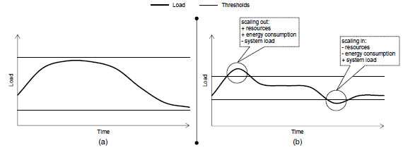
Today, the combination of horizontal and reactive approaches represents the most-used methodology for delivering cloud elasticity [4, 5, 6, 7]. In this approach, rule-condition-action statements with upper and lower load thresholds occur to drive the allocation and consolidation of instances, either nodes or virtual machines (VMs). Despite being simple and intuitive, this method requires programmer’s technical skills for tuning the parameters. Moreover, these parameters can vary according to the application and the infrastructure. Specifically for the High-performance Computing (HPC) panorama, the upper threshold defines for how long the parallel application should run close to the overloaded state. For example, a value close to 75% implies always executing the HPC code in a non-saturated environment, but paying for as many instances (and increasing energy consumption) as needed to reach this situation. Conversely, a value near to 100% for this threshold is relevant for energy saving when analyzing the number of allocations. However, this could result in weaker application reactivity, which can generate penalties in execution time. The lower threshold, in turn, is useful for deallocating resources, whereas a value close to 0% will delay this action. This scenario can cause overestimation of resource usage because the application will postpone consolidations [8]. The main reason for that behavior in HPC and dynamic applications is to avoid VM deallocations because, in a near term, the application could increase its need for CPU capacity, forcing another time-costly allocation action. Figure 1 shows two different situations resulted by different threshold organizations: (a) the load (either CPU load, network consumption or a combination of metrics, for instance) does not violates the thresholds and; (b) the load violates both thresholds resulting in elasticity operations.
Some recent efforts have specifically focused on exploiting the elasticity of clouds for traditional services, including a transactional data store, data-intensive web services and the execution of a bag-of-tasks application [9]. Basically, this scenario covers companies aiming at avoiding the downfalls involved with the fixed provisioning on mission critical applications. Thus, the typical elasticity organization on such systems uses virtual machines (VMs) replication and a centralized dispatcher. Normally, replicas do not communicate among themselves and the premature crash of each one does not mean a system unavailability, but an user request retry [10].
Although the aforementioned solution is successfully employed on server-based applications, tightly-coupled HPC-driven scientific applications cannot benefit from the use of these mechanisms. Generally, these scientific programs have been designed to use a fixed number of resources, and cannot explore elasticity without an appropriate support. In other words, the simple addition of instances and the use of load balancers have no effect in these applications since they are not able to detect and use these resources [11]. Technically, over recent years most parallel applications have been developed using the Message Passing Interface (MPI) 1.x, which does not have any support for changing the number of processes during the execution [12]. While this changed with MPI version 2.0, this feature is not yet supported by many of the available MPI implementations [9]. Moreover, significant effort is needed at application level both to manually change the process group and to redistribute the data to effectively use a different number of processes. Furthermore, the consolidation (the act of turning off) a VM running one or more processes can incur in an application crash, since the communication channels among the processes are suddenly disconnected.
Aiming at providing cloud elasticity for HPC applications in an efficient and transparent manner, we propose a model called AutoElastic (Project website: http://autoelastic.github.io/autoelastic). Efficiency is addressed at both time and energy management perspectives on changing from one resource configuration to another to handle modifications in the workload. Moreover, transparency is addressed by providing cloud elasticity at middleware level. Since AutoElastic is a PaaS-based (Platform as a Service) manager, the programmer does not need to change any line of the application’s source code to take profit of new resources. The proposed model specifically assumes that the target HPC application is iterative by nature,  , it has a time-step loop. This is a reasonable assumption for most MPI programs, so this does not limit the applicability of our framework. AutoElastic’s contributions can be divided in two ways as follows:
- Elastic infrastructure for HPC applications to provide asynchronous elasticity, both for not blocking any processes when instantiating or consolidating VMs and for managing the change on the number of processes avoiding any possibility of application crash;
- Taking into account the AutoElastic’s reactive behavior, we analyzed the impact of different upper and lower threshold values and four load patterns (constant, ascending, descending and wave) on cloud elasticity when executing a scientific application compiled using the AutoElastic prototype.
This article describes the AutoElastic model and its prototype, developed to run over the OpenNebula private cloud platform. Furthermore, it presents the rationales on AutoElastic evaluation, the implementation of a numerical integration application and a discussion about its performance with cloud elasticity. The remainder of this article will first introduce the related work in Section 2. Section 3 is the main part of the article, describing AutoElastic together with its application model in detail. Evaluation methodology and results are discussed in Sections 4 and 5. Finally, Section 6 emphasizes the scientific contribution of the work and notes several challenges that we can address in the future.
2 Related Work
Cloud computing is addressed both by providers with commercial purposes and open source middlewares, as well as academic initiatives. Regarding the first group, the initiatives in the Web offer elasticity either manually when considering the user viewpoint [13, 14, 15] or through preconfiguration mechanisms for reactive elasticity [3, 10, 16]. In particular, in the latter case, the user must setup thresholds and actions of elasticity, which may not be trivial for those not experts in cloud environments. Systems such as Amazon EC2 http://aws.amazon.com, Nimbus http://www.nimbusproject.org and Windows Azure http://azure.microsoft.com are examples of this methodology. In particular, Amazon EC2 eases the allocation and preparation of the VM but not the automatic configuration which is a requirement for a truly elastic-aware cloud platform. Concerning the middlewares for private clouds, as OpenStack https://www.openstack.org, OpenNebula http://opennebula.org, Eucalyptus https://www.eucalyptus.com and CloudStack http://cloudstack.apache.org, the elasticity is normally controlled manually, either on the command line or via a graphical application that comes together with the software package.
Academic research initiatives seek to reduce gaps and/or enhance cloud elasticity approaches. ElasticMPI proposes elasticity in MPI applications by stop-reconfigure-and-go approach [9]. Such action may have a negative impact, especially for HPC applications that do not have long duration. In addition, the ElasticMPI approach makes a change in the application’s source code in order to insert monitoring policies. Mao, Li and Humphrey [17] deal with auto-scalability by changing the number of VM instances based on workload information. In their scope, considering that a program has deadlines to conclude each of its phases, the proposal works with resources and VMs to meet these deadlines properly. Martin et al. [18] present a typical scenario of requests over a cloud service that works with a load balancer. The elasticity changes the amount of worker VMs according to the demand on the service. In the same approach of using a balancer and replicas, Elastack appears as a system running on OpenStack to address the lack of elasticity of the latter [19].
Weiwei et al. [20] use CloudSim [21] to enable dynamic resource allocations using thresholds. The resources monitoring occurs between malleable time intervals according the application regularity. Although, the application execution blocks during the resource reorganizations and there is no peak treatment when violating a threshold. This approach requires previous application information to define the thresholds. The system monitors variations in the workload to decide when resource organizations are necessary. In the tests using CloudSim, the authors used the threshold values 95%, 75% and 50%. Rui Han et al. [22] present an approach to resource management focusing IaaS (Infrastructure as a Service) to Cloud providers. The system monitors the application response time and compare the values with predetermined thresholds. When the response time reaches a threshold, the system uses horizontal and vertical elasticity to reorganize the resources. The thresholds 80% and 30% were used in the tests. Spinner et al. [23] propose an algorithm that calculates at every new application phase the ideal resource configuration based in thresholds. In this way, the approach uses vertical elasticity to increase or decrease the number of CPU’s available to the application through virtual machines. The algorithm works with a aggressiveness parameter to define the elasticity behavior. In the tests, the authors used the threshold 75%.
Chuang et al. [24] affirm that we need a model in which programmers do not need be aware of the actual scale of the application or of the runtime support that dynamically reconfigures the system to distribute application state across computing resources. To address this point, the authors developed EventWave, a programming model and runtime support for tightly coupled elastic cloud applications. The initiative focuses on a game server and works only with VM migration. Gutierrez-Garcia and Sim [25] developed an agent-based framework to address cloud elasticity for bag-of-tasks demands. The status of the BoT execution is verified every hour; if it is not completely executed, all the cloud resources are reallocated for the next hour. Wei et al. [26] explore elastic resource management on the PaaS level. When applications are deployed, they are first allocated on separate servers, so that they can be monitored more meticulously. Then, the authors collect long-term monitoring data to estimate the application’s characteristics, time that is added to the normal execution of the application. Aniello et al. [27] developed an architecture for automatically scaling replicated services. A queuing model of the replicated service is used to compute the expected response time, given the current configuration (number of replicas) and the distributions of both input requests and service times. However, a queuing system is not the best option for dynamic applications and/or infrastructure because it is based on rigid parameters. Leite et al. [28] developed a middleware named Excalibur to execute parallel applications in the cloud automatically. Excalibur works with independent tasks organized in different partitions. The algorithms must to know some information in advance, such as the total number of tasks and the estimated CPU time to execute each type of task.

Table 1 presents a comparison of the most representative works discussed in this section. Elasticity is explored further in the IaaS level as a reactive approach. In this way, the works are not unisons about the use of a single threshold for the tests. For example, it is possible to note the following values: (i) 70% [30]; (ii) 75% [31]; (iii) 80% [32]; (iv) 90% [19, 33]. These values deal with upper limits that when exceeded, trigger elasticity actions. Furthermore, an analysis of the state-of-the-art in elasticity allows to point out some weaknesses of the academy initiatives, which can be summarized in five statements: (i) no strategy is proposed to assess whether it is a peak when reach a threshold [18, 19]; (ii) need to change the application source code [9, 29]; (iii) need to know the application’s data before its execution, such as the expected time of execution of each component [9, 34]; (iv) need to reconfigure resources with stop of the application and subsequent recovery [9]; (v) supposition that the communication between VMs is given at a constant rate [35].
To summarize, in the best of our knowledge, three articles address cloud elasticity for HPC applications [9, 18, 29]. They have in common the fact that they approached the master-slave programming model. Particularly, the initiatives [9, 29] are based on iterative applications, where there is a redistribution of tasks by the master entity at each new phase. Applications that do not have an iterative loop cannot be adapted to this framework, since it uses the iteration index as execution restarting point. In addition, the elasticity in [29] is managed manually by the user, obtaining monitoring data using the framework proposed by the authors. Finally, the purpose of the solution of Martin et al. [18] is the efficient handling of requests to a Web Server. It acts as a delegator and creates and consolidates instances based on the flow of arrival requests and the load of worker VMs.
3 AutoElastic: Reactive-based Cloud Elasticity Model
This section describes the AutoElastic model, which analyzes alternatives for the following problem statements:
- 1.
- Which mechanisms are needed to provide cloud elasticity transparently at both user and application levels?
- 2.
- Considering resource monitoring and VM management procedures, how can we model the elasticity as a viable capability on HPC applications?
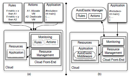
Our idea is to provide reactive elasticity totally in a transparent and effortless way to the user, who does not need to write rules and actions for resource reconfiguration. In addition, users must not need to change their parallel application, not inserting elasticity calls from a particular library or modifying the application to add/remove resources by themselves. Considering the second aforementioned question, AutoElastic should be aware of the overhead to instantiate a VM, taking this knowledge to offer this feature without prohibitive costs. Figure 2 (a) illustrates the traditional approaches of providing cloud elasticity to HPC applications, while (b) highlights AutoElastic’s idea. AutoElastic allows users to compile and submit a HPC non-elastic aware application to the cloud. So, the middleware at PaaS level firstly transforms a non-elastic application in an elastic one and secondly, it manages resource (and also application processes, consequently) reorganization through automatic VM allocation and consolidation procedures.
The first AutoElastic ideas were published in [36]. In [36], our idea was to present a deep analysis of the state-of-the-art in the cloud elasticity area, presenting the gaps in the HPC landscape. The mentioned article considered only a pair of thresholds (one upper threshold and one lower threshold), besides not explaining the interaction between the application processes and the AutoElastic Manager. Now, the current article presents a novel prediction function (see Equations 1 and 2), a graphical demonstration about how an application talks with the Manager and extensive details about the application used in the tests. Moreover, in the current article we are presenting novel types of graphs, exploring the impact of the thresholds in the application performance, the relationship between CPU load and allocated CPU cores, and energy consumption profiles.
3.1 Architecture
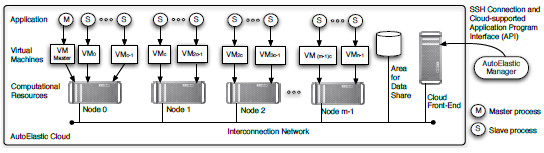
AutoElastic is a cloud elasticity model that operates at the PaaS level of a cloud platform, acting as a middleware that enables the transformation of a non-elastic parallel application in an elastic one. The model works with both automatic and reactive elasticity in their horizontal (managing VM replicas) and vertical modes (resizing computational infrastructure), providing allocation and consolidation of compute nodes and virtual machines. As PaaS proposal, AutoElastic proposes a middleware to compile an iterative-based master-slave application, besides an elasticity manager. Figure 3 (a) depicts users interaction with the cloud, who needs to concentrate their efforts only on the application coding. The Manager hides the details from the user on writing elasticity rules and actions. Figure 3 (b) illustrates the relation among processes, virtual machines and computational nodes. In our scope, an AutoElastic cloud can be defined as follows:
- Definition 1 - AutoElastic cloud: a cloud modeled with
 homogeneous and distributed computational resources, where at least one of them (Node0) is always active. This node is in charge of running a VM with the master process and other
  VMs with slave processes, where
  means the number of processing units (cores or CPUs) inside a particular node. The elasticity grain for each scaling up or down action refers to a single node, and consequently, its VMs and processes. Lastly, at any time, the number of VMs running slave processes is equal to
  .
.
Here, we are presenting the AutoElastic Manager as an application outside the cloud, but it could be mapped to the first node, for example. This flexibility is achieved by using the API (Application Programming Interface) of the cloud software packages. Taking into account that HPC applications are commonly CPU intensive [37], we opted for creating a single process per VM and  VMs per compute node to explore its fully potential. This approach is based on the work of Lee et al. [38], where they seek to explore a better efficiency in parallel applications.
 processing VMs, where
  denotes the number of processing units in the node
The user can enter an SLA (Service Level Agreement) with the minimum and maximum number of allowed VMs. If this file is not provided, it is assumed that this maximum is twice the number of VMs observed at the application launch. The fact that the Manager, and not the application itself, increases or decreases the number of resources provides the benefit of asynchronous elasticity. Here, asynchronous elasticity means that process execution and elasticity actions occur concomitantly, not penalizing the application because of resource overhead (node and VM) reconfiguration (allocation and deallocation). However, this asynchronism leads to the following question: How can we notify the application about resource reconfiguration? To accomplish this, AutoElastic communicates among the VMs and the Manager using a shared memory area. Other options of communication should also be possible, including using NFS, message-oriented middleware (such as JMS or AMQP) or yet tuple space (JavaSpaces, for instance). The use of a shared area for data interaction among VM instances is a common approach in private clouds [13, 14, 15]. AutoElastic uses this idea to trigger actions as presented in Table 2.
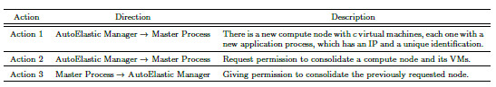
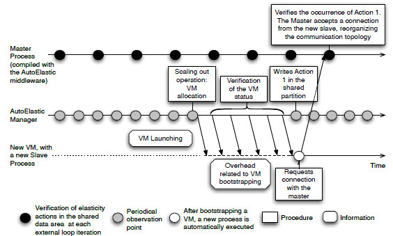
Based on Action1, the current processes may start working with the new set of resources (a single node with  VMs, each one with a new process). Figure 4 illustrates the functioning of the AutoElastic Manager when creating a new slave, so launching Action 1 afterwards. Action2 is relevant for the following reasons: (i) not stopping a process executing while either communication or computation procedures take place; (ii) ensuring that application will not be aborted with the sudden interruption of one or more processes. In particular, the second reason is important for MPI applications that run over TCP/IP networks, since they commonly crash with a premature termination of any process. Action3 is normally taken by a master process, which ensures that the application has a consistent global state where processes may be disconnected properly. Afterwards, the remaining processes do not exchange any message to the given node. We are working with a shared area because it makes easier the notification of all processes about resource addition or dropping and then, performing communication channel reconfigurations in a simple way.
AutoElastic offers cloud elasticity using the replication technique. In the activity of enlarging the infrastructure, the Manager allocates a new compute node and launches new virtual machines on it using an application template. The bootstrap of a VM is ended with the execution of a slave process which will do requests to the master. The instantiation of VMs is controlled by the Manager and only after they are running the Manager notifies the other processes through Action1. The consolidation procedure increases the efficiency on resource utilization (not partially using the available cores) and also provides a better management of energy consumption. Particularly, Baliga et al. [39] claim that the number of VMs in a node is not an influential factor for energy consumption, but the fact of a node is turned on or not.
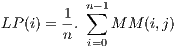
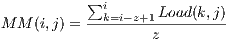
As in [16] and [31], data monitoring is given periodically. Hence, AutoElastic Manager obtains the CPU metric, applies time series based on past values and compares the final metric with the maximum and minimum thresholds. More precisely, we are employing Moving Average in accordance with Equations 2 and 1.  returns a CPU load prediction when considering the execution of the
  slave VMs in the Manager intervention number
  . To accomplish this,
  informs the CPU load of a virtual machine
  in the observation
  . Equation 2 uses moving average by considering the last
  observations of the CPU load
  over the VM
  , where
  . Finally, Action1 is triggered if LP is greater than the maximum threshold, while Action2 is thrown when LP is lower than the minimum threshold.
 | (1) |
where
 | (2) |
for  .
.
3.2 Model of Parallel Application
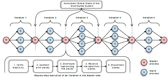
AutoElastic exploits data parallelism on iterative-based message passing parallel applications. Figure 5 shows an iterative application supported by AutoElastic where each iteration is composed by three steps: (a) the process master distributes the load among the active slave processes; (b) slave processes compute the load received by the master process; and (c) the slave processes send the computed results to the master process. The elasticity occurs always in between each iteration where the computation has a consistent global state, allowing changes in the number of processes. In particular, the current version of the model still has the restriction to operate with applications in the master-slave programming style. Although trivial, this style is used in several areas, such as genetic algorithms, Monte Carlo techniques, geometric transformations in computer graphics, cryptography algorithms and applications that follow the Embarrassingly Parallel computing model [9]. However, the Action1 allows existing processes to know the identifiers of the new ones allowing an all-to-all communication channel reorganization eventually. Another characteristic is that AutoElastic deals with applications that do not use specific deadlines for concluding the subparts.
As AutoElastic project decision, elasticity feature must be offered to programmers without changing their application. Thus, we modeled the communication framework by analyzing the traditional interfaces from MPI 1.x and MPI 2.x. The first creates processes statically, where a program begins and ends with the same number of processes. On the other hand, MPI 2.0 has support for elasticity, since it offers the possibility of creating processes dynamically, with transparent connections to the existing ones. AutoElastic follows the MPMD (Multiple Program Multiple Data) approach from MPI 2.x, where the master has an executable and the slaves another.
Based on the MPI 2.0, AutoElastic works with the following directives: (i) publication of connection ports; (ii) finding the server based on a particular port; (iii) accepting a connection; (iv) requesting a connection; (v) making a disconnection. Different from the approach in which the master process launches the slaves using a spawn-like directive, the proposed model operates according to another approach of MPI 2.0 for dynamic process management: connection-oriented communication using point-to-point, as sockets do. The launching of a VM automatically occurs in the execution of a slave process, which requests a connection with the master afterwards. Here, we emphasize that an application with AutoElastic does not need to follow the MPI 2.0 interface, but the semantic of each aforementioned directive.
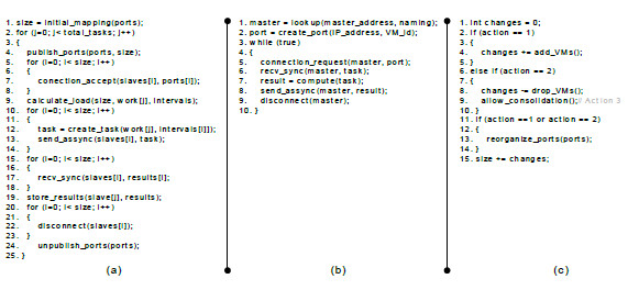
Figure 6 (a) presents a pseudo-code of the master process. The master performs a series of tasks, sequentially capturing a task and dividing it before sending for processing on slaves. Concerning the code, the method in the line 4 of Figure 6 (a) checks the distributed environment and publishes a set of ports (disjoint set of numbers, names or a combination of them) to receive a connection from each slave process. Data communication happens in an asynchronous model, where sending data to the slaves is non-blocking and receiving data from them is blocking. The occurrence of an external loop is convenient for elasticity, since the beginning of each iteration is a possible point for resource and process reconfiguration, including communication channel reorganizations. Still, the beginning of a new loop implies in a consistent global state for the distributed system.
The transformation of a non-elastic in an elastic application can be offered in different ways:
- (i)
- implementation of an object-oriented program using polymorphism to override the method to manage the elasticity;
- (ii)
- using a source-to-source translator to insert code between lines 4 and 5 of the master code;
- (iii)
- development of a wrapper for procedural languages in order to change the function in line 4 of Figure 6 (a). Regardless of the technique, the elasticity code is simple and shown in Figure 6 (c). A region of additional code checks the shared directory if there is a new action for AutoElastic. For example, this part of code can be inserted as an extension of the function publish_ports() following the technique number iii above.
Although the initial focus of AutoElastic is on master-slave, the use of the sockets-like MPI 2.0 ideas eases the inclusion of processes and the reestablishment of connections to compose a new totally arbitrary topology. At implementation level, it is possible to optimize connections and disconnections if the process persists in the list of active processes. This behavior is especially pertinent over TCP/IP connections, since this suite uses an onerous three-way hand shake protocol for connection establishment.
4 Evaluation Methodology
We developed an iterative application to execute in the cloud with different sets of load patterns and elasticity thresholds. Besides the metric application time, our idea consists in analyzing the elasticity reactivity and the costs in terms of infrastructure to achieve a particular execution time. The application computes the numerical integration of a function  in a closed interval
 ![[a,b]](/img/revistas/cleiej/v19n1/1a0123x.png) . In general, numerical integration has been used in two ways: (i) as benchmark for HPC systems, including multicore, GPU, cluster and grid architectures [40, 41]; (ii) as a computational method employed on simulations of dynamic and electromechanical systems [42, 43]. The first case explains why we are using numerical integration to evaluate the AutoElastic model. Here, we are using the Composite Trapezoidal rule from Newton-Cotes postulation [42]. Newton-Cotes formula can be useful if the value of the integrand is given at equally-spaced points. Firstly, consider the division of the interval
. In general, numerical integration has been used in two ways: (i) as benchmark for HPC systems, including multicore, GPU, cluster and grid architectures [40, 41]; (ii) as a computational method employed on simulations of dynamic and electromechanical systems [42, 43]. The first case explains why we are using numerical integration to evaluate the AutoElastic model. Here, we are using the Composite Trapezoidal rule from Newton-Cotes postulation [42]. Newton-Cotes formula can be useful if the value of the integrand is given at equally-spaced points. Firstly, consider the division of the interval ![[a,b]](/img/revistas/cleiej/v19n1/1a0124x.png) in
in  equally-spaced subintervals, each one with length
  (
(![[x ,x ] i i+1](/img/revistas/cleiej/v19n1/1a0127x.png) , for
, for  ). Thus,
  . The integral of
  is defined as the sum of the areas of the
  trapezoids contained in the interval
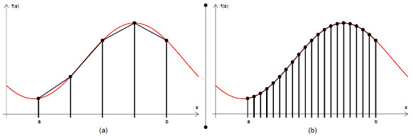
 ![[a,b]](/img/revistas/cleiej/v19n1/1a0132x.png) as presented in Equation 3. Figure 7 shows two examples of splitting the interval [a,b]: in (a) with 4 and in (b) with 20 trapezoids. Considering this figure, we can observe that the larger the number of trapezoids, or subintervals, the greater the precision to the precision to compute the total area in [a,b].
as presented in Equation 3. Figure 7 shows two examples of splitting the interval [a,b]: in (a) with 4 and in (b) with 20 trapezoids. Considering this figure, we can observe that the larger the number of trapezoids, or subintervals, the greater the precision to the precision to compute the total area in [a,b].
 | (3) |
where  = area of trapezoid
  , with
  .
.
![∫ b h- x∑-1 a f(x)dx ≈ 2[f(x0)+ f(xs) +2. f (xi)] i=1](/img/revistas/cleiej/v19n1/1a0137x.png) | (4) |
Equation 4 shows the development of the numerical integration in accordance with the Newton-Cotes postulation. This equation is used to develop the parallel application modeling. The values of  and
and  in Equation 4 are equal to
  and
and  , respectively. In this context,
  means the number of subintervals. Following this Equation, there are
 -like simple equations for getting the final result of the numerical integration. The master process must distribute these
  equations among the slaves. Logically, some slaves can receive more work than others when
  is not fully divisible by the number of slaves. As being defined in
  the amount of subintervals to compute the integration, the greater this parameter, the larger the computational load involved on reaching the result for a particular equation.
Aiming at analyzing the impact of different thresholds in the parallel application, we used the aforesaid parameter  to model four load patterns: Constant, Ascending, Descending and Wave. An execution of a load consists in start the application with a set of integral equations with the same parameters and a different
  for each one. In each iteration the master process distributes the load of one equation. Varying the parameter
  we can increase or decrease the load for each equation. Table 3 shows the function used to calculate the load for each equation in each iteration. The idea of using different patterns, or workloads, for the same HPC application is widely explored in the literature to observe how the input load can impact in points of saturation, bottlenecks and resource allocation and deallocation [44, 45, 46].
 ,
,  is the iteration index at application runtime
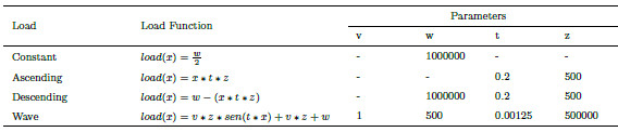
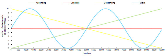
Figure 8 shows a graphical representation of each pattern. The  axis in the graph of Figure 8 expresses the functions (each iteration represents a function) that are being tested, whereas the
  axis informs the respective load. Again, the load represents the number of subintervals
  between limits
  and
and  , which in this experiment are 1 and 10, respectively. A greater number of intervals is associated with a greater computational load for generating the numerical integration of the function. For simplicity, the same function is employed in the tests, but the number of subintervals for the integration varies.
The loads were executed in two different scenarios: (i) starting with 2 nodes and (ii) starting with 4 nodes. We are using 2.9 GHz dual core nodes with 4 GB of RAM memory and an interconnection network of 100 Mbps. Each load was executed against each scenario when considering AutoElastic with and without enabling the elasticity feature. In the case where the elasticity is active, all loads were tested  times, where
  is the number of combinations of maximum and minimum possible thresholds. Assuming the choices of different works, where we can find thresholds like 50% [47], 70% [30][47], 75% [31], 80% [33][47] and 90% [19][47], for the maximum value, we adopted 70%, 75%, 80%, 85% and 90%, while the minimum thresholds were 30%, 35%, 40%, 45% and 50%. Particularly, the range for the minimum threshold is based on the work of Haidari et al. [47], who propose a theoretical analysis with queuing theory to observe cloud elasticity performance.
 | (5) |
 | (6) |
Besides the performance perspective, we also analyze the energy consumption in order to perceive the impact of the elasticity feature. In other words, we do not want to reduce the application time by using a large number of resources, thus consuming much more energy. Empirically, we are using Equation 5 for estimating the energy consumption. This equation relies on the close relationship between energy and resource consumption as presented by Orgerie et al. [48]. In this context, we use Equation 5 to create an index of the resource usage. Here, we use the same ideas of the pricing model employed by Amazon and Microsoft; they consider the number of VMs at each unit of time, which is normally set to an hour.  presents the time that the application executed with
  virtual machines. Therefore, our unit of time depends on the measure of
  (in minutes, seconds or milliseconds, and so on) in which the final intent is to sum the number of VMs used at each unit of time. For example, considering a unit of time in minutes and an application completion time of 7 min, we could have the following histogram: 1 min (2 VMs), 1 min (2 VMs), 1 min (4 VMs), 1 min (4 VMs), 1 min (2 VMs), 1 min (2 VMs) and 1 min (2 VMs). Finally, 2 VMs were used in 5 min (partial resource equal to 10) and 4 VMs in 2 min (partial resource equal to 8), summing to 18 for Equation 5. Thus, Equation 5 analyzes the use from
  to
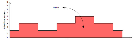
to  VMs, considering the partial execution time on each infrastructure size. To the best of our understanding, the energy index here is relevant for comparison among different elastic-enabled executions. Figure 9 represents the energy consumption as an area calculation. Taking into account both our measure of energy (see Equation 5) and the application time, we can evaluate the cost
  by multiplying both aforementioned values (see Equation 6). The final idea consists of obtaining a better cost when enabling the AutoElastic’s elasticity feature in a comparison with an execution of a fixed number of processes.
5 Discussing the Results
This section shows the results obtained when executing the parallel application in the cloud considering two scenarios:
- (i)
- using AutoElastic, enabling its self-organizing feature when dealing with elasticity;
- (ii)
- using AutoElastic, considering scheduling computation, but without taking any elasticity action. Particularly, the values of thresholds are not important in this second scenario since infrastructure reconfiguration does not take place.
Subsection 5.1 presents an analysis of the impact on the application time when varying the threshold configuration. The results concerning energy consumption and cost to execute the application are presented in the Subsection 5.2.
5.1 Impact of the Thresholds on Application Time
Aiming at analyzing the impact and possible trends of the employed thresholds on application time, we organized the results in the Figures 10 and 11. Both present the final execution time when enabling elasticity and maximum and minimum thresholds. At performance perspective, we observed that the time is not significantly changed when varying the minimum threshold (see the lower part of the Figures 10 and 11). On the other hand, the maximum threshold impacts in the application performance directly, where the larger the maximum threshold the larger the execution time. The lack of reactivity is the main cause for this situation,  , the application will execute in the overloaded stated during a larger period when evaluating thresholds close to 90%. Particularly, this behavior is more evident when using the Ascending function. In this case, the workload grows up continuously and then, a threshold close to 70% can allocate more resource faster, relieving the system CPU load quickly too.
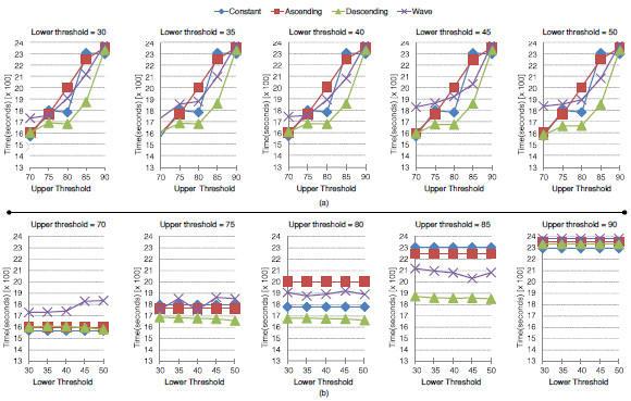
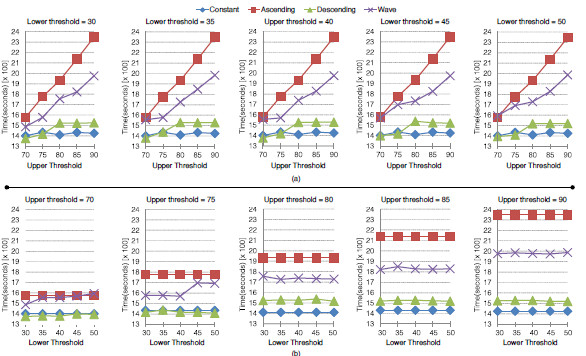
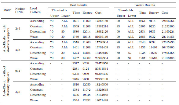
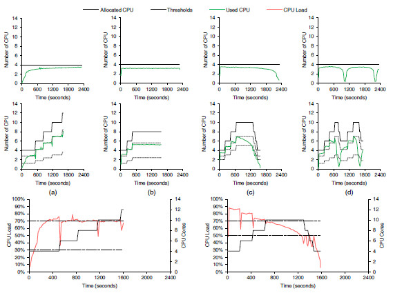
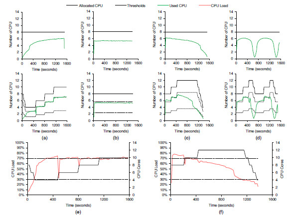
Table 4 presents the results for the best and the worst execution times when varying the used load patterns and the scenarios. In addition, Figures 12 and 13 illustrate the performance involving the column of the best results under the two aforementioned scenarios. Each node starts with two VMs, each one running a slave process in one of two cores of the node. Considering that the application is CPU-bound, the execution with 4 nodes outperforms about 65% in average the tests with 2 nodes without enabling elasticity. This explains also the better results with elasticity when considering the start configuration with 2 and 4 nodes. In other words, the possibility to change the number of resources has a stronger impact when initializing a more limited configuration. For example, Figure 12 (a) shows the Ascending function and the increment up to 12 CPUs (6 nodes) with elasticity, denoting a performance gain up to 31%. Here, we can observe that the used CPU reaches the total allocated quickly, demonstrating the application’s CPU-bound character. Considering this figure and the Descending function, we allocate up to 10 CPUs that become underutilized, being deallocated close to the final of the application. This occurs because AutoElastic does not work with previous knowledge of the application, acting only with data captured at runtime.
5.2 Energy Consumption and Cost
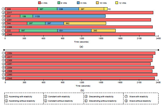
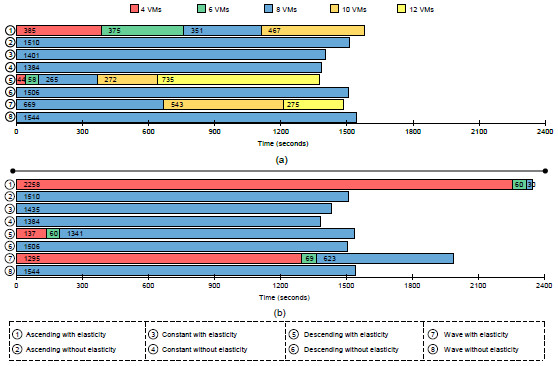
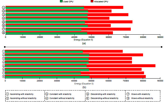
Figures 14 and 15 present an application execution profile, depicting the mapping of VMs when considering the best and worst results (see Table 4). The start with 2 nodes (4 VMs) does not present elasticity actions in the worst case when using the maximum threshold equal to 90%. This explains the results in the part (b) of Figure 14. Yet with 2 nodes in the starting moment, threshold 70% is responsible for allocating up to 12 VMs in the Ascending load as we can observe in Figure 14 (a). Contrary to this situation, Figure 15 shows less variation on resource configuration, when 4 nodes (or 8 VMs) are maintained in the larger part of the execution. As exception, we can observe the Ascending function as the worst case, where a maximum threshold equal to 90% is employed. The application starts reducing the number of VMs from 8, to 6 up 4, using this last value in 96% of the execution. Although not exceeding a load of 90%, so not enlarging the infrastructure, the allocation of more resource in this situation could help on both balancing the load among the CPUs and reducing the application time.
Figure 16 illustrates the amount of allocated and used CPU considering the best cases of f 4. All loads used less CPU when enabling the elasticity, except in the Constant load when starting with 4 nodes which we achieved the same value in both cases. However, the use of 2 nodes as start configuration implies on allocating more CPU when enabling elasticity. This behavior was expected for two reasons: (i) AutoElastic does not use a prior information about application behavior; (ii) after allocating resources, the overall load decreases implying on a better load balancing but on a worse resource utilization.
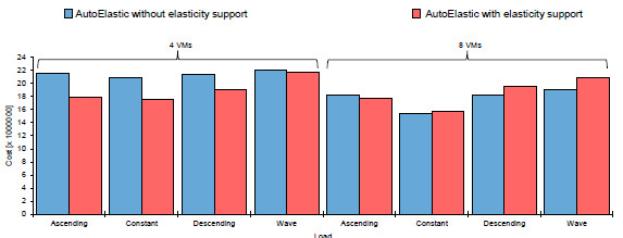
Considering the Figures 14 (a) and 15 (a), we computed the energy consumption as declared in Equation 5. Considering this metric and the application time, we can configure the cost as previously mentioned in Equation 6. The final idea regarding the cost is summarized in the Inequality 7, where our plan is either to reduce the time but not paying a large resource penalty for this or to present a time slightly larger than a non-elastic execution but improving resource utilization. In this Inequality,  means the scenario with AutoElastic and elasticity, while
  means the scenario with same middleware but resource reconfiguration does not take place. Figure 17 illustrates the cost results when starting with 2 and 4 nodes. Elasticity is responsible for the better results in the former case over all evaluated loads. On the other hand, the lack of reactivity and static thresholds were the main reasons for the results in the latter case. In other words, the application executes inefficiently during a large period up to reaching a threshold, so implying after this on resource reconfiguration. The prediction of application behavior and adaptable thresholds could aid to improve performance when using configurations with a reduced computation grain (index that can be estimated by dividing the work involved on computational tasks by the costs on network communication).
 | (7) |
6 Conclusion
This article presented a model named AutoElastic and its functioning in the HPC scope when varying both the cloud elasticity thresholds and the application’s load pattern. Considering the problem statements (listed in Section 3), AutoElastic acts at middleware level targeting message-passing applications with explicit parallelism, which use send/receive and accept/connect directives. Particularly, we adopted this design decision because it can be easily implemented in MPI 2, which offers a sockets-based programming style for dynamic process creation. Moreover, considering the time requirements of HPC applications, we modeled a framework to enable a novel feature denoted asynchronous elasticity, where VM transferring or consolidation happens in parallel with application execution.
The main contribution of this work is the joint analysis of an elasticity model and a HPC application when varying both elasticity parameters and load patterns. Thus, the discussion here can help cloud programmers to tune elasticity thresholds to exploit better performance and resource utilization on CPU-driven demands. At a glance, the gain with elasticity depends on: (i) the computational grain of the application; (ii) elasticity reactivity. We showed that a CPU-bound application can execute faster with elasticity when comparing its execution with other scenarios which use a fixed and/or reduced number of resources. Considering this kind of applications, we observed that a maximum threshold (that drives the infrastructure enlargement) close to 100% can be seen as a bad choice because the application will execute unnecessarily with overloaded resources up to reach this threshold level. In our tests, our lower value for this parameter was 70%, which had generated the best results over all load patterns.
Future research concerns the study of network, storage and memory elasticity to employ these capabilities in the next versions of AutoElastic. Moreover, we plan to develop a hybrid proactive and reactive strategy for the elasticity, joining ideas from reinforcement learning, neural networks and/or time-series analysis. Future works also include investigations on designing the SLA. Today, we are considering only the maximum number of VMs, but metrics like time, energy and cost can be also combined in this context. The study of elasticity grain and the execution of highly irregular applications also contemplate future steps. The grain, in particular, refers to the number of nodes and VMs involved on each elasticity action. Regarding the target application, although the numerical integration application be useful to evaluate AutoElastic ideas, we intend to explore elasticity on highly-irregular applications [49]. Our plans also consider to extend AutoElastic to cover elasticity on other HPC programming models, such as divide-and-conquer, pipeline and bulk-synchronous parallel (BSP). In addition, the current article focused mainly on exploring the impact of the lower and upper thresholds in the application performance; so future work also includes the development of 3D graphs in order to demonstrate their impact also in the energy and cost perspectives.
Acknowledgment
The authors would like to thank to the following Brazilian agencies: CNPq, CAPES and FAPERGS.
References
[1] M. Mohan Murthy, H. Sanjay, and J. Anand, “Threshold based auto scaling of virtual machines in cloud environment,” in Network and Parallel Computing, ser. Lecture Notes in Computer Science, C.-H. Hsu, X. Shi, and V. Salapura, Eds. Springer Berlin Heidelberg, 2014, vol. 8707, pp. 247–256.
[2] J. Bao, Z. Lu, J. Wu, S. Zhang, and Y. Zhong, “Implementing a novel load-aware auto scale scheme for private cloud resource management platform,” in Network Operations and Management Symposium (NOMS), 2014 IEEE, May 2014, pp. 1–4.
[3] S. Sah and S. Joshi, “Scalability of efficient and dynamic workload distribution in autonomic cloud computing,” in Issues and Challenges in Intelligent Computing Techniques (ICICT), 2014 International Conference on, Feb 2014, pp. 12–18.
[4] A. Weber, N. R. Herbst, H. Groenda, and S. Kounev, “Towards a resource elasticity benchmark for cloud environments,” in Proceedings of the 2nd International Workshop on Hot Topics in Cloud Service Scalability (HotTopiCS 2014), co-located with the 5th ACM/SPEC International Conference on Performance Engineering (ICPE 2014). ACM, March 2014.
[5] P. Jamshidi, A. Ahmad, and C. Pahl, “Autonomic resource provisioning for cloud-based software,” in Proceedings of the 9th International Symposium on Software Engineering for Adaptive and Self-Managing Systems, ser. SEAMS 2014. New York, NY, USA: ACM, 2014, pp. 95–104. [Online]. Available: http://doi.acm.org/10.1145/2593929.2593940
[6] Y. Guo, M. Ghanem, and R. Han, “Does the cloud need new algorithms? an introduction to elastic algorithms,” in Cloud Computing Technology and Science (CloudCom), 2012 IEEE 4th International Conference on, December 2012, pp. 66 –73.
[7] G. Galante and L. C. E. d. Bona, “A survey on cloud computing elasticity,” in Proceedings of the 2012 IEEE/ACM Fifth International Conference on Utility and Cloud Computing, ser. UCC ’12. Washington, DC, USA: IEEE Computer Society, 2012, pp. 263–270.
[8] A. Beloglazov, J. Abawajy, and R. Buyya, “Energy-aware resource allocation heuristics for efficient management of data centers for cloud computing,” Future Gener. Comput. Syst., vol. 28, no. 5, pp. 755–768, May 2012. [Online]. Available: http://dx.doi.org/10.1016/j.future.2011.04.017
[9] A. Raveendran, T. Bicer, and G. Agrawal, “A framework for elastic execution of existing mpi programs,” in Proceedings of the 2011 IEEE Int. Symposium on Parallel and Distributed Processing Workshops and PhD Forum, ser. IPDPSW ’11. Washington, DC, USA: IEEE Computer Society, 2011, pp. 940–947.
[10] P. Jamshidi, A. Ahmad, and C. Pahl, “Autonomic resource provisioning for cloud-based software,” in Proceedings of the 9th International Symposium on Software Engineering for Adaptive and Self-Managing Systems, ser. SEAMS 2014. New York, NY, USA: ACM, 2014, pp. 95–104. [Online]. Available: http://doi.acm.org/10.1145/2593929.2593940
[11] E. F. Coutinho, G. Paillard, and J. N. de Souza, “Performance analysis on scientific computing and cloud computing environments,” in Proceedings of the 7th Euro American Conference on Telematics and Information Systems, ser. EATIS ’14. New York, NY, USA: ACM, 2014, pp. 5:1–5:6. [Online]. Available: http://doi.acm.org/10.1145/2590651.2590656
[12] R. R. Expósito, G. L. Taboada, S. Ramos, J. Touriño, and R. Doallo, “Evaluation of messaging middleware for high-performance cloud computing,” Personal Ubiquitous Comput., vol. 17, no. 8, pp. 1709–1719, Dec. 2013. [Online]. Available: http://dx.doi.org/10.1007/s00779-012-0605-3
[13] B. Cai, F. Xu, F. Ye, and W. Zhou, “Research and application of migrating legacy systems to the private cloud platform with cloudstack,” in Automation and Logistics (ICAL), 2012 IEEE International Conference on, August 2012, pp. 400 –404.
[14] D. Milojicic, I. M. Llorente, and R. S. Montero, “Opennebula: A cloud management tool,” Internet Computing, IEEE, vol. 15, no. 2, pp. 11 –14, March-April 2011.
[15] X. Wen, G. Gu, Q. Li, Y. Gao, and X. Zhang, “Comparison of open-source cloud management platforms: Openstack and opennebula,” in Fuzzy Systems and Knowledge Discovery (FSKD), 2012 9th International Conference on, May 2012, pp. 2457 –2461.
[16] D. Chiu and G. Agrawal, “Evaluating caching and storage options on the amazon web services cloud,” in Grid Computing (GRID), 2010 11th IEEE/ACM International Conference on, October 2010, pp. 17 –24.
[17] M. Mao, J. Li, and M. Humphrey, “Cloud auto-scaling with deadline and budget constraints,” in Grid Computing (GRID), 2010 11th IEEE/ACM International Conference on, October 2010, pp. 41 –48.
[18] P. Martin, A. Brown, W. Powley, and J. L. Vazquez-Poletti, “Autonomic management of elastic services in the cloud,” in Proceedings of the 2011 IEEE Symposium on Computers and Communications, ser. ISCC ’11. Washington, DC, USA: IEEE Computer Society, 2011, pp. 135–140.
[19] L. Beernaert, M. Matos, R. Vilaça, and R. Oliveira, “Automatic elasticity in openstack,” in Proceedings of the Workshop on Secure and Dependable Middleware for Cloud Monitoring and Management, ser. SDMCMM ’12. New York, NY, USA: ACM, 2012, pp. 2:1–2:6. [Online]. Available: http://doi.acm.org/10.1145/2405186.2405188
[20] W. Lin, J. Z. Wang, C. Liang, and D. Qi, “A threshold-based dynamic resource allocation scheme for cloud computing,” Procedia Engineering, vol. 23, no. 0, pp. 695 – 703, 2011, pEEA 2011.
[21] R. N. Calheiros, R. Ranjan, A. Beloglazov, C. A. F. De Rose, and R. Buyya, “Cloudsim: a toolkit for modeling and simulation of cloud computing environments and evaluation of resource provisioning algorithms,” Software: Practice and Experience, vol. 41, no. 1, pp. 23–50, 2011. [Online]. Available: http://dx.doi.org/10.1002/spe.995
[22] R. Han, L. Guo, M. M. Ghanem, and Y. Guo, “Lightweight resource scaling for cloud applications,” Cluster Computing and the Grid, IEEE International Symposium on, vol. 0, pp. 644–651, 2012.
[23] S. Spinner, S. Kounev, X. Zhu, L. Lu, M. Uysal, A. Holler, and R. Griffith, “Runtime vertical scaling of virtualized applications via online model estimation,” in Proceedings of the 2014 IEEE 8th International Conference on Self-Adaptive and Self-Organizing Systems (SASO), September 2014.
[24] W.-C. Chuang, B. Sang, S. Yoo, R. Gu, M. Kulkarni, and C. Killian, “Eventwave: Programming model and runtime support for tightly-coupled elastic cloud applications,” in Proceedings of the 4th Annual Symposium on Cloud Computing, ser. SOCC ’13. New York, NY, USA: ACM, 2013, pp. 21:1–21:16. [Online]. Available: http://doi.acm.org/10.1145/2523616.2523617
[25] J. O. Gutierrez-Garcia and K. M. Sim, “A family of heuristics for agent-based elastic cloud bag-of-tasks concurrent scheduling,” Future Gener. Comput. Syst., vol. 29, no. 7, pp. 1682–1699, Sep. 2013. [Online]. Available: http://dx.doi.org/10.1016/j.future.2012.01.005
[26] H. Wei, S. Zhou, T. Yang, R. Zhang, and Q. Wang, “Elastic resource management for heterogeneous applications on paas,” in Proceedings of the 5th Asia-Pacific Symposium on Internetware, ser. Internetware ’13. New York, NY, USA: ACM, 2013, pp. 7:1–7:7. [Online]. Available: http://doi.acm.org/10.1145/2532443.2532451
[27] L. Aniello, S. Bonomi, F. Lombardi, A. Zelli, and R. Baldoni, “An architecture for automatic scaling of replicated services,” in Networked Systems, ser. Lecture Notes in Computer Science, G. Noubir and M. Raynal, Eds. Springer International Publishing, 2014, pp. 122–137.
[28] A. F. Leite, T. Raiol, C. Tadonki, M. E. M. T. Walter, C. Eisenbeis, and A. C. M. a. A. de Melo, “Excalibur: An autonomic cloud architecture for executing parallel applications,” in Proceedings of the Fourth International Workshop on Cloud Data and Platforms, ser. CloudDP ’14. New York, NY, USA: ACM, 2014, pp. 2:1–2:6. [Online]. Available: http://doi.acm.org/10.1145/2592784.2592786
[29] D. Rajan, A. Canino, J. A. Izaguirre, and D. Thain, “Converting a high performance application to an elastic cloud application,” in Proceedings of the 2011 IEEE Third International Conference on Cloud Computing Technology and Science, ser. CLOUDCOM ’11. Washington, DC, USA: IEEE Computer Society, 2011, pp. 383–390.
[30] W. Dawoud, I. Takouna, and C. Meinel, “Elastic vm for cloud resources provisioning optimization,” in Advances in Computing and Communications, ser. Communications in Computer and Information Science, A. Abraham, J. Lloret Mauri, J. Buford, J. Suzuki, and S. Thampi, Eds. Springer Berlin Heidelberg, 2011, vol. 190, pp. 431–445.
[31] S. Imai, T. Chestna, and C. A. Varela, “Elastic scalable cloud computing using application-level migration,” in Proceedings of the 2012 IEEE/ACM Fifth International Conference on Utility and Cloud Computing, ser. UCC ’12. Washington, DC, USA: IEEE Computer Society, 2012, pp. 91–98.
[32] M. Mihailescu and Y. M. Teo, “The impact of user rationality in federated clouds,” Cluster Computing and the Grid, IEEE International Symposium on, vol. 0, pp. 620–627, 2012.
[33] B. Suleiman, “Elasticity economics of cloud-based applications,” in Proceedings of the 2012 IEEE Ninth International Conference on Services Computing, ser. SCC ’12. Washington, DC, USA: IEEE Computer Society, 2012, pp. 694–695.
[34] T. Knauth and C. Fetzer, “Scaling non-elastic applications using virtual machines,” in Cloud Computing (CLOUD), 2011 IEEE International Conference on, July 2011, pp. 468 –475.
[35] X. Zhang, Z.-Y. Shae, S. Zheng, and H. Jamjoom, “Virtual machine migration in an over-committed cloud,” in Network Operations and Management Symposium (NOMS), 2012 IEEE, April 2012, pp. 196 –203.
[36] R. d. R. Righi, V. F. Rodrigues, C. A. da Costa, G. Galante, L. C. E. de Bona, and T. Ferreto, “Autoelastic: Automatic resource elasticity for high performance applications in the cloud,” IEEE Transactions on Cloud Computing, vol. 4, no. 1, pp. 6–19, Jan 2016.
[37] F. Azmandian, M. Moffie, J. Dy, J. Aslam, and D. Kaeli, “Workload characterization at the virtualization layer,” in Modeling, Analysis Simulation of Computer and Telecommunication Systems (MASCOTS), 2011 IEEE 19th International Symposium on, July 2011, pp. 63–72.
[38] Y. Lee, R. Avizienis, A. Bishara, R. Xia, D. Lockhart, C. Batten, and K. Asanovic, “Exploring the tradeoffs between programmability and efficiency in data-parallel accelerators,” in Computer Architecture (ISCA), 2011 38th Annual International Symposium on, 2011, pp. 129–140.
[39] J. Baliga, R. Ayre, K. Hinton, and R. Tucker, “Green cloud computing: Balancing energy in processing, storage, and transport,” Proceedings of the IEEE, vol. 99, no. 1, pp. 149–167, 2011.
[40] K. Banas and F. Kruzel, “Comparison of xeon phi and kepler gpu performance for finite element numerical integration,” in Proceedings of the 2014 IEEE Intl Conf on High Performance Computing and Communications, 2014 IEEE 6th Intl Symp on Cyberspace Safety and Security, 2014 IEEE 11th Intl Conf on Embedded Software and Syst (HPCC,CSS,ICESS), ser. HPCC ’14. Washington, DC, USA: IEEE Computer Society, 2014, pp. 145–148. [Online]. Available: http://dx.doi.org/10.1109/HPCC.2014.27
[41] K. A. Hawick, D. P. Playne, and M. G. B. Johnson, “Numerical precision and benchmarking very-high-order integration of particle dynamics on gpu accelerators,” in Proc. International Conference on Computer Design (CDES’11), no. CDE4469. Las Vegas, USA: CSREA, 18-21 July 2011, pp. 83–89.
[42] M. Comanescu, “Implementation of time-varying observers used in direct field orientation of motor drives by trapezoidal integration,” in Power Electronics, Machines and Drives (PEMD 2012), 6th IET International Conference on, 2012, pp. 1–6.
[43] E. Tripodi, A. Musolino, R. Rizzo, and M. Raugi, “Numerical integration of coupled equations for high-speed electromechanical devices,” Magnetics, IEEE Transactions on, vol. 51, no. 3, pp. 1–4, March 2015.
[44] S. Islam, K. Lee, A. Fekete, and A. Liu, “How a consumer can measure elasticity for cloud platforms,” in Proceedings of the third joint WOSP/SIPEW international conference on Performance Engineering, ser. ICPE ’12. New York, NY, USA: ACM, 2012, pp. 85–96. [Online]. Available: http://doi.acm.org/10.1145/2188286.2188301
[45] M. Mao and M. Humphrey, “Auto-scaling to minimize cost and meet application deadlines in cloud workflows,” in Proceedings of 2011 International Conference for High Performance Computing, Networking, Storage and Analysis, ser. SC ’11. New York, NY, USA: ACM, 2011, pp. 49:1–49:12. [Online]. Available: http://doi.acm.org/10.1145/2063384.2063449
[46] Y. Zhang, W. Sun, and Y. Inoguchi, “Predict task running time in grid environments based on cpu load predictions,” Future Generation Computer Systems, vol. 24, no. 6, pp. 489 – 497, 2008. [Online]. Available: http://www.sciencedirect.com/science/article/pii/S0167739X07001215
[47] F. Al-Haidari, M. Sqalli, and K. Salah, “Impact of cpu utilization thresholds and scaling size on autoscaling cloud resources,” in Cloud Computing Technology and Science (CloudCom), 2013 IEEE 5th International Conference on, vol. 2, Dec 2013, pp. 256–261.
[48] A.-C. Orgerie, M. D. D. Assuncao, and L. Lefevre, “A survey on techniques for improving the energy efficiency of large-scale distributed systems,” ACM Computing Surveys, vol. 46, no. 4, pp. 1–31, Mar. 2014. [Online]. Available: http://dl.acm.org/citation.cfm?doid=2597757.2532637
[49] L. Jin, D. Cong, L. Guangyi, and Y. Jilai, “Short-term net feeder load forecasting of microgrid considering weather conditions,” in Energy Conference (ENERGYCON), 2014 IEEE International, May 2014, pp. 1205–1209.

