


Servicios Personalizados
Revista

Articulo
 Inglés (pdf)
 Articulo en XML
 Referencias del artículo
Links relacionados
Compartir

 Permalink
CLEI Electronic Journal
versión On-line ISSN 0717-5000
CLEIej vol.18 no.2 Montevideo ago. 2015
Let’s go to the cinema! A movie recommender system for ephemeral groups of users
Abstract
Going to the cinema or watching television are social activities that generally take place in groups. In these cases, a recommender system for ephemeral groups of users is more suitable than (well-studied) recommender systems for individuals. In this paper we present a recommendation system for groups of users that go to the cinema. The system uses the Slope One algorithm for computing individual predictions and the Multiplicative Utilitarian Strategy as a model to make a recommendation to an entire group. We show how we solved all practical aspects of the system; including its architecture and a mobile application for the service, the lack of user data (ramp-up and cold-start problems), the scaling fit of the group model strategy, and other improvements in order to reduce the response time. Finally, we validate the performance of the system with a set of experiments with 57 ephemeral groups.
Abstract in Spanish or Portuguese
Ir al cine, o ver la televisión, son actividades sociales que por lo general se llevan a cabo en grupos. En estos casos, un sistema de recomendaciones para grupos efímeros de usuarios es más adecuado que los (bien estudiados) sistemas de recomendaciones para individuos. En este trabajo se presenta un sistema de recomendaciones para grupos de usuarios que van al cine. El sistema utiliza el algoritmo ”Slope One” para calcular predicciones individuales y una estrategia utilitaria multiplicativa para unificar esas predicciones en una recomendacion grupal. Mostramos cómo solucionamos todos los aspectos prácticos del sistema; incluyendo su arquitectura y una aplicación móvil para el servicio, los problemas que surgen de la falta de datos de usuarios, los problemas de escalamiento, y otras mejoras con el fin de reducir el tiempo de respuesta. Finalmente, validamos el rendimiento del sistema con un conjunto de experimentos con 57 grupos efímeros.
Keywords: recommender systems, ephemeral group recommendation, collaborative filtering, Slope One, utilitarian strategy.
Keywords in Spanish:sistemas de recomendación, grupos efímeros, filtros colaborativos, Slope One, estrategia utilitaria.
Submitted: 2014-11-11. Revised: 2015-04-07. Accepted: 2015-07-12.
1 Introduction
In recent years consumption of on-demand multimedia content over the Internet has greatly increased, with a great deal of contents available through streaming platforms and services such as Netflix [1], YouTube [2, 3], Amazon Instant Video [4], Hulu [1], Crackle [5](for video streaming) or Spotify [6], Deezer [7], Google Play Music [8], Napster [9] (for music streaming), to name only a few. While this is positive, it is more difficult for the consumer to choose the most suitable content for its preference. Be able to suggest and to arrange somehow this content, and facilitate the user the task of select a content from an almost infinite universe of possibilities are common objectives and current hot research topics. As shown in previous research [10], to find the best content for an individual could be a difficult problem. In this work, we study an even greater challenge: to find the best option for a set of individuals or group. Following the literature [11, 12, 13, 14, 15, 16, 17, 18], we know that the problem is more complex when the group cannot be properly characterized, for example when the group is ephemeral (i.e. there is no previous knowledge about the group and the group will dissolve in the near future).
Therefore, in this article we will board the problem of recommender systems for ephemeral groups. Specifically, we will raise the construction of a prototype of a mobile application that users can use to form ephemeral groups in order to go to the cinema; and of course, the application will help them in the selection process of what movie to watch. As explained in the following sections, our proposed prototype combines a preference prediction algorithm for individuals with a group’s recommendation strategy, in order to recommend the best movies for each group. In order to validate the performance of our recommendation system, we perform a preliminary set of experiments with 57 ephemeral groups. Obtaining promising results, getting over  of groups accept one of the three main system recommendations.
Despite that the focus of this paper is to present the developed recommendation system, we show how we solved all practical aspects of the system; including its architecture, the mobile application to offer the service, and several particular problems solved during the implementation. In the following, we present the contents of this paper.
In Section 2, we present the related work and we describe the basic concepts about recommender systems, deepening into the Slope One algorithm and the Multiplicative Utilitarian Strategy. Then, in Section 3 we present some relevant aspects of the implementation of our recommender system, including, how we solved some problems such as the ramp-up and the cold start problem, or the scaling problem intrinsic of the Multiplicative Utilitarian Strategy, and how we improved the performance of Slope One algorithm in time and storage, doing a partial load of the Slope One matrix and other variants of the basic algorithm. Section 4 presents the first calibrations and performance evaluations of our recommender system. In Section 5, we show an end-user oriented mobile application designed to leverage the recommender system. Users can create events (going to the cinema), invite other users to join the event, receive recommendations about a cinema listing, and evaluate individual or group predictions. We evaluate the performance of the application in Section 6. With the help of more than  experiments with real groups of users (of size between
  and
and  individuals), we validate the effectiveness and efficiency of our prototype. Last, in Section 7 we resume the main conclusions of the work.
2 Related Work
Large work has been done in recommender systems for individuals. In [10], Ricci, F. et al. distinguishes between six different classes of recommendation approaches based on different knowledge sources: content-based, collaborative filtering, demographic, knowledge-based, community-based and hybrid. This classification, which provides a taxonomy that has become a classical way of referring to and distinguishing among recommender systems for individuals, can be summarized as follows [10]:
- Collaborative Filtering: it is considered the most popular and widely implemented technique. It provides recommendations using only information about rating profiles for different users. In one of its forms, since there are some variants which will be discussed later in this section, this technique locates peer users with a rating history similar to the current user and provides recommendations using this notion of neighborhood. In this work we will use a collaborative filtering technique, and this class will be introduced in next Subsection 2.1.
- Content-based: it provides recommendations from two sources: the features associated with items and the ratings that the user has given them. It learns to recommend items that are similar to the ones that the user liked in the past. The similarity of items is computed based on the features associated with the compared items. Therefore, the recommendation problem is solved as a user-specific classification problem and it learns a classifier for the user’s likes and dislikes based on item features.
- Demographic: it generates recommendations based on a demographic profile of the user. Recommended items can be provided for different demographic niches, by combining the ratings of users in those niches.
- Knowledge-based: it provides recommendations based on inferences about the user’s profile. Usually, this knowledge is provided to the particular case, and sometimes contain explicit functional knowledge about how certain item features meet user needs.
- Community-based: it is a new type of recommendation technique based on the preferences of the users friends. It performs well in special cases, when items (or users) are highly dynamic, or when the user ratings of specific items are highly varied (i.e. controversial items).
Also, the taxonomy adds an extra Hybrid technique that combines these pure techniques in order to improve accuracy or efficiency comparing it with each technique separately. For example, since all the learning-based techniques (collaborative filtering, content-based and demographic) suffer from the cold-start problem (described in Section 3), the combination with a knowledge-based technique makes it possible to reduce the impact of that problem. For a detailed explanation of possible hybrid techniques, please read [19].
2.1 Collaborative Filtering Recommender Systems for users
Recommender systems using collaborative filtering technique (CFRS) take ratings made by users over items as input for the recommendation algorithm. They consider the ratings assigned by the user for whom the recommendation is being generated and the recommendations made by the other users. CFRS relate two different entities: items and users. Traditionally, there have been two main approaches to facilitate such a comparison: model-based methods and neighborhood methods [10, 20]. These approaches are presented in the next subsections. Also, some others works have been implemented in order to solve some problems that traditional algorithms have had in particular contexts. In subsection 2.1.3 we dedicated some lines to them.
2.1.1 Model-based methods
They use the gathered information to make an off-line model which is then used to make predictions more efficiently [21]. Cluster Model, Latent Factor models and Bayesian Networks are some alternatives of this approach. In [21], you can find a complete description and a study that compares them. It is worth noting, that Cluster Model, for instance, reaches a complexity order of  for the prediction function [22]. Latent Factor models, such as matrix factorization (aka, singular value decomposition), is a new approach of CFRS that transforms both, items and users, to the same latent factor space [23, 24, 15]. The latent space tries to explain ratings by characterizing both items and users on factors automatically inferred from ratings. Recent studies show that this approach has a high accuracy, and offers a number of practical advantages.
2.1.2 Neighborhood methods
They focus on the notion of similarity (the neighborhood) of items or, alternatively, of users. The neighborhood of a user is built from users whose profiles are similar to his or her profile, considering ratings on common items that are shared by them to make the comparison. Similarly, the neighborhood of an item is the set of other items similar to it, and the comparison is based on common ratings that users have made. Accordingly, the rating of an item for a given user can be predicted based on the ratings given by the neighborhood of users and items. In [22], Candillier et. al. explain that there are two main approaches within CF Neighborhood methods: user-based, and item-based.
User-based and item-based approaches use the notion of neighborhood between users and items respectively to compute the predicted rating of a user over an item. There are different measures of similarity to assess how similar a pair of users or a pair of items are. A similarity measure is presented as a measure of relevance between two vectors. When values of these vectors are related to a user model, it is called user-based similarity measure; otherwise, it is called item-based similarity measure [25]. With respect to the computation, the main difference between user-based and item-based approaches is how the vectors are taken from the user-item matrix of ratings. In the first case, the similarity is computed over the rows of the matrix, while in the second, the calculation is performed over the columns [26]. Some most used similarity measures used are: Pearson Correlation, Cosine Vector, Adjusted Cosine Vector, Quadratic Difference, Simple Matching Coefficient, Jaccard Coefficient, Extended Jaccard (Tanimoto) Coefficient, Spearman Rank Correlation, Mean Squared Difference, Minkowski distance (where Euclidean distance is a particular case), the City Block metric, and the Supremum distance. Historically, Pearson Correlation has been generally recognized as the best similarity measure [10], but recent investigations show that the performance of such measures depended greatly on the data [10]. In our work we have implemented the Slope One algorithm, which unlike other collaborative filter algorithms, does not handle the concept of similarity. For that reason, we will not go into detail about the similarity measures mentioned above. You can read about it in detail in [10].
2.1.3 Other approaches for CFRS
In particular contexts, traditional algorithms have had some problems, sometimes making almost impossible to execute quickly, in real-time and without losing quality. For that reason some variations in collaborative filtering have appeared. The Slope One algorithm and the Amazon’s item-to-item Collaborative Filtering are two examples of these new approaches. The item-to-item Collaborative Filtering was implemented by Amazon after testing and realizing that traditional algorithms did not perform well enough with their massive data sets (tens of millions of customers and millions of distinct catalog items). Unlike traditional collaborative filtering, the computation for the Amazon’s algorithm scales independently of the number of customers and number of items. It produces recommendations in real-time, scales to massive data sets, and generates high quality recommendations [27]. Rather than matching the user to similar customers, item-to-item collaborative filtering matches each of the user’s purchased and rated items to similar items, then combines those similar items into a recommendation list [28]. Both, the Slope One and the item-to-item algorithms, use an offline computed item-to-item matrix in order to generate recommendations quickly and in real time. In the case of the item-to-item algorithm this matrix maintains the information for knowing how similar are items between them. On the other hand, the Slope One algorithm uses an item-to-item matrix for knowing how much more an item is liked over another item on average. Because for computing the entries of the matrix, both algorithms consider only users who have rated (or purchased in the case of the item-to-item algorithm) both items, then the recommendation is very quick, depending only on the number of items that the user has purchased or rated. You can deepen in the item-to-item algorithm in [27] and [28]. The next subsection explains the algorithm used in our work: Slope One.
2.2 Slope One algorithm
Slope One is a family of algorithms from the CFRS category that tries to solve some of the common problems that have other recommendation algorithms. It was introduced in 2005 by Daniel Lemire and Anna Maclachlan in [29]. That paper lists the five main objectives of the algorithm:
- Easy to deploy and maintain. Easy to interpret.
- Instant update. If new ratings arrive, all predictions are changed instantly.
- Efficient at query time. Queries can be executed quickly, the cost is the storage space it requires.
- Users with few recommendations, will receive good recommendations.
- Reasonable accuracy with simplicity and ability to scale.
Several studies [29, 30, 31, 32] show that these objectives are reached: it offers excellent quality (with a performance closer to the best known recommender algorithm, including common user-based and item-based approaches), and it needs the lowest computational time. Consequently, the Slope One algorithm was chosen for this work.
According to its authors, the algorithm operates under the principle of differential popularity between items (instead of handle the concept of similarity). This principle can be defined as the average of rating differences, indicating how much more an item is liked over another item on average, considering for the calculation only those users who rated both items. For example, if we have  items in our system, and the users who have rated items
  are
are  , we define the ratings vector for user
  as
as 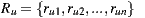 where
where  represents the rating of user
  over the item
  . Then, if we have
  and
and  the average ratings are
  (
( ) and
) and  (
( ) for
) for  and
and  respectively. Then, the average of rating differences for both items is
  (only considering the ratings given by users who have rated both items). This difference can be understood as a 1-point advantage of
  over
over  .
.
Slope One uses this average of rating differences to predict the rating a user would give to an item that has not yet rated. Considering the values of the previous example, if we know that a user has rated  with
with  , then we would predict the rating over
  with a value of
  , maintaining the linear relationship between the two items (
 is liked in average one point more than
  ). If we repeat this reasoning considering all the items the user has already rated and the average of rating differences for these items against the item to predict, then we could refine the prediction value for the user by averaging predictions resulting from consider each of the items already rated. Now, with this consideration we formally present the Slope One prediction function for a user
  over an item
  with this formula:

where  represents all items rated by user
  except item
  ,
,  represents the rating for user
  over the item
  , and
, and  represents the average of deviation for ratings considering items
  and
and  , which is calculated using the following formula:
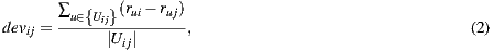
where  denotes the set of users who rated both items
  and
and  ,
,  is the number of users in the set,
  and
and  the ratings of user
  over the items
  and
and  respectively.
To meet the goal of being efficient at query time, the implementations of Slope One perform an off-line pre-processing stage to build an initial matrix with the  values computed for all pair of items
  and
and  for which there are at least one user who has rated them both. This matrix can be updated quickly each time a new rating arrives [29]. Thus, considering that the rest of the prediction formula is computed on-line, all predictions are changed instantly, thus fulfilling the goal that refers to the instant update.
The above paragraphs explain the basic scheme of Slope One computation. As detailed in the original work of Slope One [29], there are at least two other schemes to show: the Weighted Slope One scheme and the Bi-Polar Slope One scheme. In the Weighted Slope One scheme, the popularity of the items, i.e. the known ratings, are taken into account. The basic assumption is that if we have more ratings about an item, we can predict with better accuracy using this item. To exemplify this point, let us assume that we want to predict the rating over the item  by a user
  , and we know that the user
  rated items
  and
and  . If there are much more users that rated both
  and
and  against
  and
and  , it makes more sense to expect better confidence in the linear relationship between
  and
and  than the relationship between
  and
and  . This idea is not encompassed in the prediction Equation (1), which can be improved consequently through the following weighted formula:
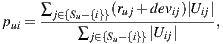
where  denotes the number of users who rated both items
  and
and  .
.
The Bi-Polar Slope One scheme is an improvement over the Weighted Slope One scheme, that takes into account the confidence of ratings over pairs of items (as the weighted version), and a bi-polar classification (like/dislike) of users over items. Formally, we split the rating set of user  ,
,  , into two sets of rated items:
 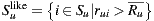 and
and 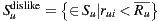 , where
  is the average rating values provided by user
  . Also, the set of users who rated both items
  and
and  ,
,  , is splitted accordingly:
  and
and 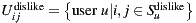 . Using these splitted sets, the Bi-Polar Slope One scheme restricts the set of ratings that are used in the prediction and deviation formulas. First, in the deviation formula (improve over Equation (2)), only deviations between two liked items or deviations between two disliked items are taken into account:
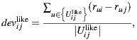
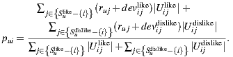
a similar equation defines  . Second, in the prediction formula (improve over Equation (1)), only deviations from pairs of users who rated both item
  and
and  and who share a like or dislike of item
  are used to predict ratings for item
  :
:
As explained in Section 3, we will use a new variant of the basic scheme (inspired in the weighted version) that reduces the amount of items considered for computation, in order to improve performance. As our set of items is relatively small, a premise of our work was to not develop the solution over big-data software, like in [30], in order to obtain portability and fast scripting programming.
2.3 Group Recommender Systems
Unlike other activities such as using the computer, reading a book or listening to music, going to the cinema or watching television are social activities that generally take place in groups. Livingstone & Bovill in their research report called Young people, new media [33] state that television is the medium that is more frequently shared with the family, topping the list of activities that parents share with their children, and also that more than two thirds of children watch their favorite shows with someone else, usually a family member. Therefore, in this context, it is essential to have recommender systems that generate recommendations for an entire group of individuals.
Compared with recommender systems for individuals, few systems have been developed that take into account a set of individuals to generate recommendations [12, 11]. One of these is PolyLens [13] (extension of MovieLens), a research project from the Minnesota University that recommended movies for small groups of users. The study of PolyLens has helped to understand the considerations that must be taken into account when developing systems for groups. Another highly recognized system in this category is MusicFX [34], whose main objective is to select radio stations in a fitness club. To choose the radio station, MusicFX takes into account the preferences of musical genres of those who are developing their workout at that time. Some other known systems that generate recommendations for groups are: Intrigue (recommends places for groups of tourists), The Travel Decision Forum and The Collaborative Advisory Travel System (both help a group of users to choose a joint holiday), and YU’S TV recommender (TV program recommender for groups), you can read more about them in [10].
In [14], Bernier et. al. explain the two main approaches for providing recommendations to a group of users: group model based and individual recommendation merging. These approaches differ from each other on how the recommender applies aggregation of individual information.
In the case of Individual Recommendation Merging, an individual recommendation is made for each group member and then the results are aggregated [14, 15, 16]. The purpose of this approach is to present a set of items to the entire group that be the merging of the items preferred by each member of the group [17]. An algorithm that implements this approach typically will have two stages. In a first stage, for each group member, the system predicts the user’s rating on each item that the user has not yet rated and the set of items  with the highest prediction is selected. Finally, in the second stage, the list of items to recommend to the group is constructed as the merging of the
  of each member [17].
In our work we have chosen a Group Model Based approach in order to implement a group recommendation strategy, by building the group profile using the individual profile of each member of the group. With this approach, a group recommender system considers the preferences of each individual in the group with some criterion that maximizes the happiness of the group (also called group’s satisfaction). The concept of group happiness can vary, it sometimes corresponds to the average of preferences of the members, and other times to the happiest (and least happy) member, etc.. There are different strategies (many of them inspired by the Social Choice Theory and the Voting Theory [12, 18, 35, 36]) and different algorithms to compute the happiness value according to the definition we use. All these algorithms have as their main input the individual satisfaction prediction for users who make up the group. The work in [14] classifies the recommendation strategies in the following categories: majority-based (consider only the most popular items), consensus-based (consider all group member preferences), and borderline (consider only a subset of items, belonging to a subgroup of members). Below, we describe some strategies with outstanding features as representatives of this categorization: plurality voting, the least misery, the most respected person, and utilitarian.
2.3.1 Plurality voting
This strategy also known as first past the post (or by its initials PPTP or FPP) belongs to the majority-based classification according to [14]. We present it because of its simplicity and intuitiveness. Each person votes for his or her preferred alternative, then the alternative with the most number of ratings wins. If required to choose a set of alternatives, the method can be repeated, firstly to choose the first alternative, then voting for the second, and so on. A disadvantage of this strategy is that it violates the Condorcet Winner Criterion which is one of the desirable properties of social choice procedures [36].
An alternative meets the Condorcet Winner Criterion if when compare it with each of the others, is the preferred one. More formally, given the alternatives 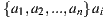 is an alternative that meets the Condorcet Winner Criterion if for all
  such that
 , then
  . Given this definition, consider the following scenario in a hypothetical election:
- 30% prefer
 before
  before
- 30% prefer
 before
  before
- 40% prefer
 before
  before
If we apply the Plurality Voting strategy, then  would be the winning option with 40% of the votes, although 60% prefers
  before
  . This simple example shows that while alternative
  is the winner,
  is not the most preferred alternative and shows clearly the disadvantage of this strategy to violate the Condorcet Winner Criterion.
2.3.2 The least misery
This strategy was chosen in the design of PolyLens [13] and belongs to the borderline classification according to [14]. For each alternative, the lowest rating given by any individual is considered, then the results are sorted in descending order and the alternative that tops the list is the winner. The idea of this strategy is that the happiness of the group is dictated by the happiness of the least happy member. While in small groups it could be a good alternative, it has the disadvantage that for large groups it could happen that an item is never chosen as the winner because there is one member who hates it, despite the fact that a huge majority would love it [37, 38].
2.3.3 The most respected person
This strategy also known as Dictatorship belongs to the borderline classification according to [14]. We find it interesting to mention this strategy because, despite its simplicity, it has performed very well in the evaluation of different strategies according to [39], only improved by the utilitarian strategy. The strategy consists in considering only the ratings given by the most respected person in the group, without regard to the ratings or opinions of the rest. That would be a typical scenario when a guest is watching TV with the usual members of a family or when it is the birthday of any individual in the group [12].
2.3.4 Utilitarian
This strategy takes its foundations from the Utilitarianism ethical theory, which has been used in different areas and disciplines such as philosophy, economics or political science. The Utilitarianism, as an ethical theory, holds that any action should seek the greatest happiness for the greatest number of individuals and that actions which are right in proportion to that tend to promote happiness [40]. It is important to note that to apply this approach, it might be necessary to take an action that does lose happiness to few individuals with the objective of maximizing overall happiness. This is a problem to be faced by individuals who enjoy greater happiness when applying this theory and that few are able to consent. Stuart Mill in [40] summarizes this problem with its famous phrase ”It is better to be a human being dissatisfied than a pig satisfied; better to be Socrates dissatisfied than a fool satisfied”.
In order to apply these principles in a group recommendation strategy, utility values are used to measure the happiness of each individual in each alternative. These values generally correspond to the ratings assigned (if they are known) or individually predictions for the alternative. There are two versions of this strategy, the additive and multiplicative, and both belong to the consensus-based classification according to [14]. In the additive utilitarian version, the sum of the utility values for each individual is computed for each alternative. Alternatives are then sorted in descending order according to the result of the sum. We should note that if we perform the average of the utility values for each alternative, the order of the list remains the same, so this strategy is also known as the Average strategy [41]. The item that tops the list is the one that maximizes the happiness of the group (note that it could possibly be more than one) and, by generalizing, we say that if an item  is before an item
  in the list, then
  is more recommendable for the group than
  , according to this strategy. In the multiplicative utilitarian version, the product of the utility values for each individual is computed for each alternative. Alternatives are then sorted in descending order according to the result of the product. Although this version is very similar to the additive version, the result list can be very different as can be seen in the example summarized in Table 2.
2.3.5 Analysis of the strategies
 predicted for three users

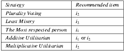
Table 2 summarizes these four group strategies with an example to see which item would be the recommended in each case. Suppose three users  for whom the system predicts the values
  ,
,  and
and  respectively on the item
  , and
, and  ,
,  , and
, and  on the item
  , as shown in the Table 1. Also suppose that
  is the most respected person in the group. If we decide to use the Plurality Voting strategy then
  would be the winner because
  is the first option for
  and
and  , and only
  would prefer
  instead of
  . If the Least Misery strategy is used then
  would be the winner too, in this case because the lowest prediction for
  is 1 and for
  is 2, so when the lowest values for each alternative are ordered in descending,
  is at the head of the list, so it is the winner option. In case of using The Most Respected Person strategy and supposing that
  is the most respected person,
  would be the recommended item because is the preferred option for
  . Finally, if we apply the Additive Utilitarian strategy for both items we get the value of
  to express the happiness of the group, creating a draw in the value of the prediction on both items. In contrast, if we use the Multiplicative Utilitarian strategy we get a happiness value of
  for
for  and
and  for
for  , breaking the draw in the happiness values that are predicted.
Unlike other strategies such as the Least Misery and the Average Without Misery, Utilitarian strategy has the disadvantage (in both versions: additive and multiplicative) that minorities are not taken into account. This is worse in big groups, because in small groups each individual opinion has a large impact [12, 14]. On the other hand, the Utilitarian strategy is the one that has achieved the best results in the evaluation of different strategies according to [39]. In particular, multiplicative strategy is the best performing strategy, according to [41] and [10]. Moreover, it provides adequate privacy for individuals [42], which is another desirable feature for a group recommendation strategy [42]. For these reasons, the multiplicative utilitarian strategy was the one we have chosen to implement in our work.
Finally, to end this section on group recommendations devote a few paragraphs to the privacy issues for groups of individuals.
2.3.6 Privacy considerations
Privacy is an important factor to generate recommendations for groups, especially if, in pursuit of transparency, the system indicates that a particular item is shown because a particular member of the group is interested in it [42]. The use of personal data may be disclosed or not to users. Different implementations could deal with this issue in different ways, such as making this information available to users, leaving the control to each individual user or hiding it completely [13]. Few studies and experiments have been aimed at the study of privacy in group recommendations. Two of the most important works on the subject are PolyLens [13], and the investigation performed by Judith Masthoff and Albert Gatt in [42]. In [13], reaction of users to loss of privacy was studied. In PolyLens, most groups were small, many compounds for close friends, so privacy was not a major problem and users were willing to yield some privacy to get the benefits of group recommendations. Finally, [13] concludes that more work is required in the future to understand the behavior of other types of groups.
[42] investigates the effect on privacy of different group aggregation strategies and describes three methods to improve privacy. The first one consists in giving the user the possibility to indicate the degree of privacy (between 0 and 1) of each rating given to each item. The second one is about providing the ability to use different user profiles depending on the situation and context (individual, family, friends, etc). The third method consists in the use of anonymity. [42] concludes that using the Least Misery strategy should be avoided and indicates it is fine to use the multiplicative utilitarian strategy. Finally, [42] proposes to add a virtual member (with their own tastes) to the group in order to improve privacy. Thus, it would add a bit of casuistry to the recommendations, and the result of a recommendation could never be attributed to a particular individual because there is always the possibility that it has been influenced by the virtual user.
3 Our Cinema Recommender System
Justified by previous works, we decide to use the Slope One algorithm in order to predict individual recommendations, and combine them into a group recommendation using the multiplicative utilitarian strategy. In this Section, we present the most relevant implementation details of our recommendation system. Firstly, we present the Ramp-up and Cold Start problems, that are two intrinsic problems to recommender systems and the solution we implemented. Then, we continue to present another problem, specific to the Slope One algorithm, and referring to the big data process required in order to compute the matrix of rating differences. We show some relevant properties about this matrix and how we took advantage of them in order to perform a partial load of this matrix, with the aim of reducing the recommendation time and the required space to less than a half. Finally, we consider a variation for the Slope One algorithm in order to improve the recommendation time and we show an intrinsic scaling fit problem of multiplicative utilitarian strategy and a possible solution for dealing with it.
3.1 Ramp-Up and Cold Start problems
The Ramp-Up problem [43] occurs when, in a newly launched system, there is insufficient information to generate good recommendations. That is, the system must know about the decisions of users to ensure the quality of future recommendations. CFRS suffer from this problem because they receive as input the history of user ratings on items. Similarly, while the system is running at steady state, Cold Start happens when a new user arrives at the system without any previously rated item, making it difficult for the system to infer his preferences.
To solve these problems we make an initial load using the MovieLens 10M dataset [44], with data from anonymous users, items and scores. Once this dataset is loaded, we use these data to initialize the matrix of average of rating differences used by the Slope One algorithm. Thus, taking advantage of the benefits of the Slope One algorithm, new users must just rate a few movies when they enter the system for the first time (Figure 1), so that the algorithm can find entries in the matrix of average of rating differences and start generating good recommendations for the user.
3.2 Partial load for the Slope One Matrix
As mentioned in Section 2.2, Slope One algorithm uses as its input a matrix of size  x
x , where
  is the number of items in the system. In a movies domain,
  can be very large. For example, the MovieLens 10M dataset [44] has more than
  movies (and it only considers movies until 2009), therefore, the matrix should have more than
  million entries. This is the price that Slope One pays in order to make recommendations in an efficient way, but it can become a problem if you do not have good storage capacity or if you have limitations on the size of the used database. For example, in this work, we use a SQL Server Express 2008 R2 database which limits the database size to 4GB. For this reason we decided to perform a partial load of the matrix, as follows.
Each element of the matrix used by Slope One indicates how much more an item is liked than another on average, specified by  , and is computed according to Equation (2). It is easy to see that
  and
and  happen for all item
  and
and  . These properties classify our matrix as an antisymmetric matrix, since it is a square matrix which fulfills that its transpose is equal to its negative (
 ). This observation is important because it allows us to load only the upper part of the matrix, because the rest of the values can be computed.
To perform the initialization process, we built an application that iterates over all movies in the MovieLens 10M dataset [44], and for each one, computes and stores the value of average of rating differences with the rest of the movies that have a greater identifier. To consider only greater identifiers ensures us that only the upper part of the matrix will be loaded (given the antisymmetric property), and it allows us to save significant space for storage and to reduce the size of the matrix to less than a half, which also helps us to improve performance of queries to solve the prediction algorithm and therefore the recommendations.
3.3 Variant for the Slope One algorithm
The Equation (1) specifies the predicted rating of user  over the item
  ,
,  . In this computation, we can see that the number of items rated by the user affects the execution time of the algorithm. If we define
  as the size of set
  , the formula for
  has
has  . If we use a lower value for
  , the number of operations will be less. On the other hand, the Weighted Slope One algorithm [29] weighted the most rated movies, assuming that these can contribute to a better result. Following this approach, we reduce the set
  , re-defined as
  , where
  is the subset of items from
  that have the greatest number of ratings. In Section 4 we analyze the performance of the algorithm and the prediction time, taking the size of
  as the main variable. Thus, in the rest of this document, we will use the prediction,
  , defined as:

3.4 Scaling problem of Multiplicative Utilitarian Strategy
The algorithm that we used to generate group recommendations from individual recommendations is the multiplicative utilitarian. This is so because this algorithm has performed well in similar scenarios, and because it preserves the privacy of individual ratings [42]. For this strategy, we use  prediction as utilitarian value for a user
  over an item
  . In this way we define the happiness prediction function (or satisfaction) of the group
  over an item
  as:
as:

If we compute the group happiness on a set of items, we can establish an order of preference of the group on that set of items. If ordered in descending preference, we obtain the recommendation for one or more items for the group  . Thus, we have solved the recommendation of items for a group.
Since in our system users rate movies and receive individual predictions on a scale of  , and as individual prediction is the utilitarian value for the group strategy, we can see that the minimum value of happiness for
  is
is  and its maximum value is
  , where
  is the number of members of the group
  . This is a problem, because we want that the prediction for the group has the same range of values on a scale of
  . Therefore, we have to define a new function
  as the average rating prediction (between 1 and 5) for a group
  over an item
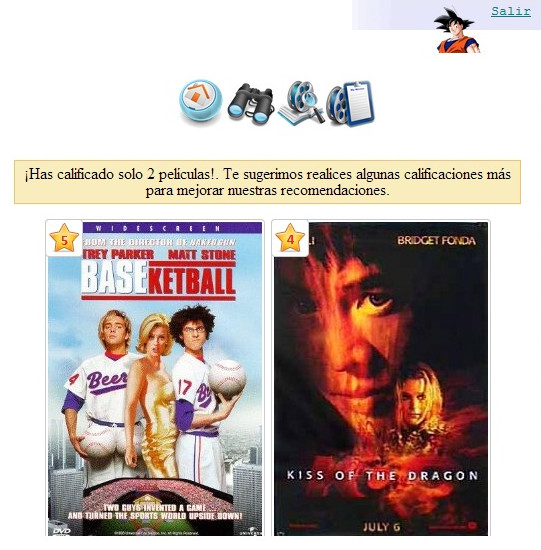
  . Then, we can try to compute the average concept of a sum at the product level, which is known as geometric mean. The geometric mean of a set of
  positive numbers is the
  root of the product of all the numbers in the set. It has the advantage that considers all distribution values and extreme values have less influence than on the arithmetic mean. It has the disadvantage that it is not determined if any value in the set is
  or if the result of the product is negative and the cardinality of the set is even. Anyway, these potential drawbacks do not apply to our context because the possible values to multiply are always between
  and
and  . Therefore, in this work, the group prediction equation takes the form:
where  is the number of users in the group.
4 Recommender System Calibration and Performance
Our main objective is to get a good group recommendation in near real-time. As we said before, in order to implement the group recommendation strategy we use the multiplicative utilitarian strategy, which considers the preference of each individual in the group by calculating the product of the individual predictions as the happiness value for the group. Therefore, the individual prediction algorithm strongly determines the final total time for the recommendation. Next, we will detail the experimental results obtained when studying the following measures:
- performance of the individual prediction algorithm,
- total time to solve the final recommendation for the entire group (expressed in
 format).
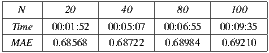
In order to measure the performance of the individual prediction algorithm, we used the Mean Absolute Error (MAE). MAE is a metric that measures the average deviation between the prediction for users over items and the real rating that those users enter to the system. It is formally defined as follows:

where  is the rating of user
  over item
  ,
,  is the prediction value for the same user and item, and
  is the number of elements in the set
  .
.
As a first approach to measure performance and time, we ran the algorithm to recommend  items for a group of
  users. We evaluated the results for both algorithms: the original Slope One algorithm and the variant we implemented. As expected, we observed that the total time to predict the recommendation varies with the amount of recommended items. We ran these tests using an Intel Core i7 1.6 GHz, 4GB RAM, OS Windows 7 Home Premium and a SQL Server Express 2008 R2 database. The dataset used was the MovieLens 10M dataset [44], which has the distribution presented in Table 3.

4.1 Performance of the Slope One algorithm
We ran the Slope One algorithm taking a sample of users from the full dataset, keeping the distribution percentages for ratings as shown in the Table 3. The obtained results were as follows:  and Total time
  . The error in these results is consistent with the expected error, according to previous studies in [30] and [31]. However, when we observe the time required to compute the recommendation for the entire group, we see that it is not an acceptable time for an interactive system.
4.2 Performance of the Slope One variant
As we explained in Section 3.3, with the aim of improving the response time of recommendation, we implemented a variant of the Slope One algorithm. In order to analyze the results of this implementation we took a sample of users from the full dataset, keeping the distribution percentages for ratings as shown in the Table 3 (like in the previous experiment for the common Slope One implementation). Then we define the input variable N representing the size of  in the Equation (3) (
 is the set of items with the highest number of ratings among the items that user
  has rated). By varying
  , we obtain the results shown in the Table 4.
 ) for different values of number of items
  .
.
The results show that reducing the number of ratings used in the algorithm, we can improve performance without a large cost in quality. We confirm that the total time for generating the recommendation decreases in proportion to  . Then, according to the results obtained, we decided to set the size of
  to
to  .
.
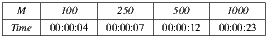
4.3 Amount of recommendable items
If we consider only the  items with the highest number of ratings among the items that user
  has rated, computing the recommendation for a group with
  users, over a catalog of
  items, has an order of
  (using the group recommendation algorithm defined in Equations (5) and (3)). Therefore, reducing
  , we get an even smaller recommendation time. As a disadvantage, we have that possible recommendations will be bounded, since we are restricting the co-domain of the recommendation function. The recommendation time for
  , taking as variable the number of items
  that can be recommended is presented in Table 5.
 and different values of number of items
  .
.
As we already mentioned, our work has as its main objective to recommend movies from cinema listings for a group of users, so  corresponds to the movies in the cinema listings for the date range in which the group intends to go to the cinema. In this way, we significantly decrease the recommendation time compared to the scenario of the whole catalog, and it validates our initial intuition on the no need of a big-data software in order to perform the task.
This approach is also applicable to other contexts than cinema listings, where the subset of candidate movies could be created from some pre-filter (e.g. gender), which allows the user to guide the recommender system, and thus preventing the system from considering those results that the user already knows will not be of interest for him or her. For other applications where the time taken to generate the recommendation is not something critical (sending weekly suggestions to users subscribed via email for example), then there would be no problem in considering the whole catalog and there would not need to limit the value of  . As we see, depending on the context for which the recommendation is used, It may make sense to consider the entire catalog or just a subset of it. Therefore, in our implementation, the set of items to recommend is an input parameter to the recommendation algorithm, which, in the specific case of going to the cinema, is the set of movies in the cinema listings within the range of dates that the group intends to go to the cinema.
5 The Mobile Application and the System Architecture
In order to test and validate our recommender system for ephemeral groups, we developed a full functional prototype that helps end-users to plan going to the cinema in group. The prototype is formed by a mobile application and a central backend, that are explained in this section.
5.1 The Mobile Application
The mobile application is designed for end-user usage of the recommender system. Users can create events (going to the cinema), invite other users to join the event, receive recommendations about a cinema listing, and evaluate individual or group predictions. It is a prototype for mobile devices which consists of a HTML5 view that accesses the system’s functionality through a RESTFul API and uses frameworks for mobile devices trying to maximize the usability and user experience. Authentication is done through username and password on the local system or using some account from a social network (e.g. Facebook). Using HTML5 allows us to improve portability, maintenance, and reduce development times, because the same HTML5 application can be run on any modern mobile device without having to reprogram (in a different language) a native client for each different type of device.

(a) Add a new event to go to the cinema in the mobile application.

(b) Details of an event in the mobile application.

(c) Information details of a movie in the mobile application.
The prototype allows users to create events. Each event defines a start and an end date that the system uses to obtain entries from movie listings within that date range and generates recommendations from these entries. The event’s owner chooses a set of users from the friend list and the system sends them an invitation to participate in the event. Then, guest users accept or reject the invitation and therefore, in this way, the ephemeral group for going to the cinema is formed. Figure 2(a) shows the interface of new events. The system predicts the rating for the ephemeral group confirmed until the time for each movie and sorts these predictions in descending order, from the most recommended to the least recommended. With each user that accepts an invitation, the system immediately updates the recommendation for the group, taking into account the preferences of the new member. Figure 2(b) shows the detail of an event and the system recommendations for the current group within the movie listings. Then, each user can see all the options from the movie listings, have access to the detailed information of each movie (Figure 2(c)), watch a trailer, read the reviews, and finally select one to watch. This information is shared with other group members. Thus, in addition to generating recommendations, the system helps the group in the final decision of which movie to watch, sharing information about preferences. In [45], it is explained that this final decision is a critical piece of information that should be managed by recommender systems. Therefore, using the system’s recommendations to the group, having the possibility to check the details of each movie from the movie listings and having shared the user preferences on the different alternatives for each member, the group decides which movie to see at the cinema. Once the event is finished, each user can rate the movie that was seen, directly from the same mobile application, providing feedback to the system through the input of new ratings. The system will use these ratings to improve future recommendations for both the user and the groups that he or she integrates.
5.2 The System Architecture
The system architecture has two main components: a generic service recommender and a movie recommendation system that uses the generic service. The generic recommender service has as its main purpose implementing the algorithms for individual and group recommendations that were previously discussed. This generic service is abstracted from any particular object type to recommend, so it recommends items in a generic way. On the other hand, the movie recommender system is in charge of context items and give a semantic domain in movies and cinema. It executes the data access components, business logic and exposes the business services through a service interface for higher layers in a service-oriented architecture (SOA).
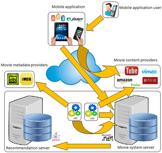
For the implementation of our prototype, we use a single server running the recommendations, but it might as well have several of these and a load balancer to scale up the solution so as to improve response times for recommendations. For example, in the case of group recommendations, the possibility of increasing these servers would allow to split group into as many subgroups as servers become available, and thus, request predictions concurrently to each server for a specific subgroup. Then, it would be sufficient to process final results in the master application server.
As shown in Figure 3, there are other important components as part of the solution. The extract, transform, and load (ETL) processes are in charge of loading meta-data and content sources from external suppliers. To achieve this, and in order to make it extensible to any other provider, we used the concept of input adapter. These adapters are responsible for getting the data from external sources, transforming them and loading them into our system using a common model structure. This common model must be well known by all adapters. As we mentioned in Subsection 5.1, each group member can check the details of the different movies in the cinema listings, as part of the help that the system provides to the group to decide which movie to see. This information has been imported by the ETL process, using meta-data from IMDB (and with the IMDbPY package [46]). Also, we keep the detail of the meta-data of each movie obtained from IMDb from the 10681 titles from Movielens, initially loaded as part of the dataset used to solve the problem of lack of data already mentioned in Section 3.1. Should be noted that mapping between IMDb and MovieLens titles is not direct. We identified two required transformations to apply to the titles obtained from MovieLens prior to searching in IMDb:
- remove the year of publication as part of the title of the movie,
- identify the occurrence of A, An, The, La, Le, Les after the title, relocate them at the beginning and remove the initial coma.
If search recovers more than one result, the identifiers are not synchronized automatically and they are stored in a temporary structure for candidates identifiers waiting to be finally resolved by human intervention. Finally, it is important to note that although this process is defined for an initial load, it also applies to synchronize new movies that are added to the cinema listings.
To implement the playback of movie trailers the system uses several ETL processes for content sources. Each adapter solves the particularities of a content supplier to extract, normalize and save the information needed to play the content, such as the input adapter of IVA Trailers which implements data access protocol Open Data Protocol (OData) to query over its data model. As part of the solution we also develop a content suppliers managment that allows to easily incorporate views for playback. It just requires to name the view with the supported supplier’s identifier. Each view knows how to interpret the information loaded by the ETL and resolves whether it must use the supplier’s player or use your own, do a redirect, mount an iframe or do whatever it takes.
Finally, in terms of communication between these components, we define a RESTFul API for communication between the mobile application and the movie recommender server, using JSON for the serialization of the exchanged messages. Communication between the movie recommender server and the generic recommender service is achieved through the use of SOAP web services.
6 Experimental Validation
In this section we will explain the tests and the results obtained when subjecting our system to recommend and make predictions to real groups of users that pretend to go to the cinema. We will begin by describing the test’s construction, then we will present the main data collected and the result obtained, both individually and for groups of users.
6.1 Test Description
6.1.1 Individuals
We invite six individuals to participate in the tests. On the main characteristics of these individuals we have that four of them are Uruguayan males: two students and two teachers of computer engineering; and two are Argentinian females outside the computer field: a music teacher and a high school student with a major in humanities. The ages range between 23 and 35. We will identify the users by the letters A, B, C, D, E and F.
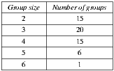
6.1.2 Groups
We make all the possible combinations of these individuals in order to generate groups of 2, 3, 4, 5 and 6 members. In total, we generate 57 groups, and Table 6 shows the number of groups by size.
 .
.
6.1.3 Cinema listings
We generate a fictitious cinema listings for 14 days. The movies for each day are taken from existing movies in the system catalog for the years 2007 and 2008. These movies correspond to the latest movies loaded into the MovieLens 10M dataset [44]. We only consider a subset of the movies for these years, the selection criterion pursued the objective of considering movies with higher amounts of information available in the system, in order to facilitate and help each individual during the process of choosing the film they prefer to see. The movie listings information included the following data: poster, title, genre, director, writer, cast, country, language, synopsis, and the link to the trailer. A total of  films are considered, with
  to
to  movies for each day.
6.1.4 Procedure
In order to avoid the cold start problem, we request each individual to rate (in the scale  ) between
  to
to  movies that they have watched previously. The movies in this training list are part of the system catalog and are not part of the test cinema listings. Once the user profile for each individual based on these initial ratings is calibrated, we send each user the following information: the groups which they belong to, the days they must go to the cinema with each group, the cinema listings for each day and the movies details. As a second stage of the test, we ask the individuals that for each day and each group, indicate us their degree of preference for each movie, also on a scale of 1 to 5 where:
- 1 = ”I wouldn’t go in no way”
- 2 = ”I wouldn’t go”
- 3 = ”Go or not is irrelevant for me”
- 4 = ”I would go”
- 5 = ”I would love to go”
An important point to note here is that this value is estimated for each individual based on the cinema listings information and trailers provided. That is, it indicates the degree of preference of the individual to go to the cinema to watch the movie with the group without actually knowing if they will like it after watching it. Later, we will use this information in order to validate our recommender system for individuals.
Finally, we ask each of the individuals, on the basis of the explicit preferences for each day and groups in which he or she participated, to indicate for each of the first three movies recommended by the system, whether they thought that the recommendation was good or not. That is, if it found that the group recommendation generated by the system is useful for the group. We also ask each individual for each day, to indicate whether their favorite movie for the day is actually the movie that the system understands is the most recommended for them. Later, we will use this information in order to validate our recommender system for groups and individuals.
6.2 Evaluation Methodology
In this section we present the methodology we have used in order to evaluate the results of our tests. First, we present the individual evaluation method used to measure whether the individual recommendations were successful or not. Second, we present a group evaluation method for the same purpose, but considering all the groups that have been formed for the test. For both, we will follow a similar approach to the T-Check method [47] used for technologies evaluation, but supplanting the design stage of a solution and the implementation of prototypes for the design and implementation of the tests we have presented in the subsection 6.1. Therefore, we will define some hypotheses that we a priori consider that should be fulfilled to consider the system useful for individuals and groups, then we will define the criteria to use in order to evaluate whether the hypotheses are fulfilled or not, and finally (and already at the next section), we will evaluate whether our hypotheses are fulfilled or not based on the tests performed and the evaluation criteria that we have defined.
6.2.1 Evaluation method for individuals
Following are the hypotheses and the evaluation criteria that we have defined to test the usefulness of our system individually. The hypothesis are:
- Individual hypothesis 1 (IH1): Predictions made by the system are similar to the explicit preferences that individuals have indicated a priori for each movie in the cinema listings.
- Individual hypothesis 2 (IH2): The movie that the system understands is the most recommended for each individual for each day, usually coincides with the movie that the individual would choose to go to watch as first choice.
And the evaluation criteria considered are:
- Evaluation criteria 1 for individual hypothesis 1 (IH1-C1): This first criterion proposes the MAE calculation for each individual and then calculating the overall MAE as an average of these. We are going to accept that the hypothesis is fulfilled if the global value for the individual MAE is similar to the expected value according to the studies of performance for the Slope One algorithm mentioned in Section 4.1, i.e. similar to
 .
. - Evaluation criteria 1 for individual hypothesis 2 (IH2-C1): This second approach is to compare for each day and each individual if the first choice that each individual chooses explicitly as the movie that they would go to see, coincides with the movie that system understand is most recommended for the individual for that day, i.e. the movie that tops the list of recommendations for the individual for that day. Then, the evaluation criterion used is based on the responses of individuals during the test when they are prompted to indicate whether their favorite movie for the day is actually the movie that the system understands is the most recommended for them. We are going to accept that the hypothesis is fulfilled based in this criterion if at least at half of the cases the system guesses the user’s first preferred option.
6.2.2 Evaluation method for groups
Following are the hypotheses and the evaluation criteria that we have defined to test the usefulness of our system at group level. The hypothesis are:
- Group hypothesis 1 (GH1): There is a high degree of acceptance in groups for system’s recommendations.
- Group hypothesis 2 (GH2): The usefulness of the system does not depend on group size. The system is useful regardless of group size (considering typical groups that goes to the cinema between 2 and 5 or 6 individuals).
And the evaluation criteria considered are:
- Evaluation criteria 1 for group hypothesis 1 (GH1-C1): This first criterion proposes the computation of the percentage of acceptance of each group that goes to the cinema to watch the movie that the system understands is the most recommended for this group based on the cinema listings for the day. We are going to accept that the hypothesis is fulfilled based in the following criterion: if at least at a half of the groups, the acceptance percentage to the system’s first recommendation reaches or exceeds half of the individuals in the group.
- Evaluation criteria 2 for group hypothesis 1 (GH1-C2): This second criterion proposes the calculation of the percentage of acceptance of each group to the movie that was the most accepted movie by individuals in the group considering the three system recommendations for this group and day. We are going to accept that the hypothesis is fulfilled based in this criterion: if at least
 of the groups, the acceptance percentage to the system’s first three recommendations reaches or exceeds half of the individuals in the group. That is, only in
  of groups the absolute majority is not reached.
 - Evaluation criteria 1 for group hypothesis 2 (GH2-C1): We will use the concept of percentile to verify that the percentages of acceptance (either to the first recommendation option or to the most accepted alternative within the three recommended items) are similar regardless of the sizes of the groups. For each group size we will plot the acceptance percentages for percentiles on a scale of 10 and we will observe the behavior of each graph. We are going to accept that the hypothesis is fulfilled based in this criterion if functional values follow the same trend for all sizes of groups plotted.
6.3 Validation and Results for Individuals
Here are the results for individuals. We present the results organized according to individual evaluation criteria that were defined in the previous section.
6.3.1 Validation of IH1-C1
For each user and entry in the cinema listings we compute the error obtained by comparing the prediction of the system vs. the explicit user preference. Figure 4 summarizes the results obtained when computing the MAE for each user individually. The overall MAE (average) is  . It is similar, but worse, than the reference value
  . The standard deviation between absolute estimations is
  , therefore our MAE is in the confidence interval of the expected value (we do not have information about confidence interval in reference works). So, we accept that the hypothesis IH1 is fulfilled based in this criterion, and therefore, we verify that the predictions made by the system for each user are similar to explicit preferences that users had indicated during the test. As a complementary information, two main differences are in our procedure compared to previous works, that would justify the deviation in MAE estimation. First, the MAE’s computation is done based on explicit preferences that individuals have indicated previously than watch the movie, and in previous works these values are the preference after watch the movie. Second, we only use 10-20 movies in order to avoid the cold start problem, where previous works have shown that they needed much more information in training stage.
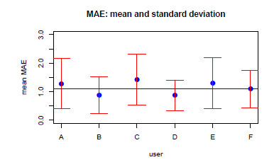
 .
.
6.3.2 Validation of IH2-C1
In order to evaluate this criterion we consider the responses of each individual during the test when they were prompted to indicate whether their favorite movie for the day was actually the movie that the system understood was the most recommended for them. Table 7 shows the users’ responses, where the computed system’s hits percentage to the first user option based on these answers is  , that does not reach the value of acceptance proposed
  (although is very close). Therefore, considering this criterion, we could not accept hypothesis IH2 as valid. Analyzing what happen, we identify that in many cases, when system does not hit which option would be the user’s first choice, we have that in general the movie that the system understands is the best option for the user, has a very close explicit preference for the option that is first choice for the user, but that because user answers only “Yes / No”, then when user marks negatively a recommendation from the system, we can not appreciate how close the system was to guess, we can only say if the system was right or not strictly, which is quite strong. Therefore, we propose to observe what happen if we modify the question, asking individuals if their first choice coincides with some of the movies that the system understands are the two most recommended movies for the individual. Now, under this new premise and as we can see in Table 8, we found that the hit’s percentage is
  surpassing the
  that we set as minimum value for the acceptance criteria. And in case of considering the three most recommended movies for the user, as seen in the Table 9, in
  of cases the system is correct that some of these films is the first choice of the individual. Given these results, we can say that our hypothesis IH2 is not valid, but the following similar hypothesis IH2’ is valid: the movie that a user would choose to go to see as first choice, usually is one of the two movies that the system understands are the most recommended for this individual and this day. This observation highlights the importance that our system should present at least the first two recommendations, and not just the first one.
 hits to the first user option. Where y means “yes, the system has guessed my first option”, n means “no, the system has not guessed my first option”, and dash - indicates that “for that day, the user did not participate in the test”.
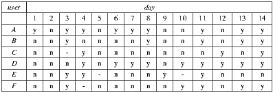
 hits to the first user option considering first two recommendations. Where y, n and - indicates the same than Table 7.
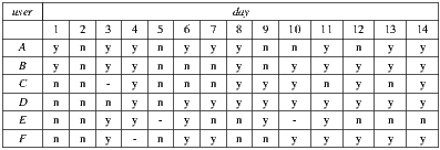
 hits to the first user option considering first three recommendations. Where y, n and - indicates the same than Table 7.
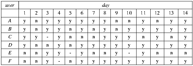
6.4 Validation and Results for Groups
6.4.1 Validation of GH1-C1
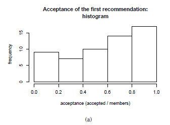
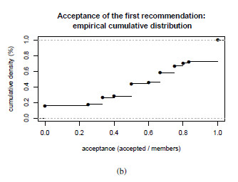
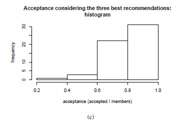
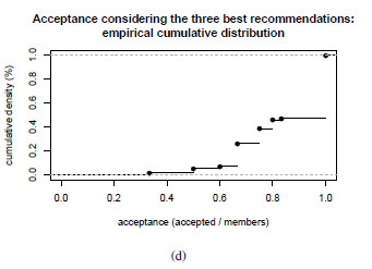
Figures 5(a) and 5(b) show the histogram and the empirical cumulative distribution of the groups’s acceptance to watch the movie that the system understands is the most recommended movie for this group.  of groups accept the first recommendation, therefore we accept that the hypothesis is fulfilled based in this criterion.
6.4.2 Validation of GH1-C2
Figures 5(c) and 5(d) show the histogram and the empirical cumulative distribution of the groups’s acceptance to watch the movie that was the most accepted movie by individuals in the group considering the three system recommendations for this group and day. As expected, a larger value of acceptance than GH1-C1 is obtained. In this case,  of groups accept one of the three main system recommendations. Therefore, we accept that the hypothesis is fulfilled based in this criterion.
6.4.3 Validation of GH2-C1
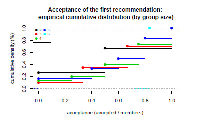
Figure 6 shows the empirical cumulative distributions (by group size) of the percentage of acceptance of each group that goes to the cinema to watch the movie that the system understands is the most recommended movie for this group. There is no change in behavior between group sizes, therefore we accept that the hypothesis is fulfilled based in this criterion.
7 Conclusion
In this paper, we present a system that recommend movies from cinema listing to ephemeral groups. To offer recommendations to ephemeral groups is a new research area and it has several practical applications beyond our particular case. In our work, we combine a group model based strategy with a collaborative filtering algorithm for individuals. As collaborative filtering we use the Slope One algorithm in order to compute individual predictions, and as group model we use the multiplicative utilitarian strategy as the technique to join predictions into a recommendation to the group.
We study in depth the application of these techniques to our specific problem, including the solution of practical problems and few improvements applicable to the particular case. As particular problems, we solve the ramp-up problem and the cold start problem, and we use the geometric mean in order to fit the scale of the multiplicative utilitarian strategy. As improvements, we implement the full system in a small server without the use of big-data software, we modify the computation of individual predictions in order to have a faster response (without loss of quality) and in order to allow the use of very useful pre-filters in the query.
We create a full prototype of the system, and we validate it in a real scenario with  groups of sizes between
  and
and  members. For this scenario, we measure the effectiveness of our solution for individual and group recommendations. We validate that our predictions for individuals are similar to the explicit preferences that individuals have indicated a priori for each movie in the cinema listings, and one of the main three recommendations coincides in
  of cases with the movie that the individual would choose to go to watch as their first choice. And more importantly, we validate that our recommendations for groups have a high degree of acceptance (
 of groups accept one of the three main system recommendations), and it does not depend on the group size (considering a typical group size of moviegoers between 2 and 6 individuals).
We expect to transform our prototype into a service, because it is close to a production software: as end-user interface we use a mobile application following the standard HTML5 with good response times, the authentication is done via common social networks, extra information about movies is downloaded from IMDb, and many other features.
References
[1] A. Banerjee, P. Rappoport, and J. Alleman, “Forecasting video cord-cutting: The bypass of traditional pay television,” in Demand for Communications Services - Insights and Perspectives, ser. The Economics of Information, Communication, and Entertainment, J. Alleman, i. M. P. NÃ-ShÃoilleabháin, and P. N. Rappoport, Eds. Springer US, 2014, pp. 59–82.
[2] J. Davidson, B. Liebald, J. Liu, P. Nandy, T. V. Vleet, U. Gargi, S. Gupta, Y. He, M. Lambert, B. Livingston, and D. Sampath, “The youtube video recommendation system,” in Proceedings of the 2010 ACM Conference on Recommender Systems, RecSys 2010, Barcelona, Spain, September 26-30, 2010, 2010, pp. 293–296. [Online]. Available: http://doi.acm.org/10.1145/1864708.1864770
[3] R. Zhou, S. Khemmarat, and L. Gao, “The impact of youtube recommendation system on video views,” in Proceedings of the 10th ACM SIGCOMM Conference on Internet Measurement 2010, Melbourne, Australia - November 1-3, 2010, 2010, pp. 404–410. [Online]. Available: http://doi.acm.org/10.1145/1879141.1879193
[4] Amazon, “Amazon instant video,” http://www.amazon.com/Instant-Video/b?node=2858778011, last access: 2015-03-29.
[5] Crackle, “Crackle home page,” http://www.crackle.com, last access: 2015-03-29. [Online]. Available: http://www.crackle.com
[6] G. Kreitz and F. Niemelä, “Spotify – large scale, low latency, P2P music-on-demand streaming,” in IEEE Tenth International Conference on Peer-to-Peer Computing, P2P 2010, Delft, The Netherlands, 25-27 August 2010, 2010, pp. 1–10. [Online]. Available: http://dx.doi.org/10.1109/P2P.2010.5569963
[7] “Deezer - Discover music you’ll love,” http://www.deezer.com/, last access: 2015-03-29. [Online]. Available: http://www.deezer.com/
[8] “Google Play Music,” https://play.google.com/music/, last access: 2015-03-29. [Online]. Available: https://play.google.com/music/listen
[9] Napster, “Rhapsody home page,” http://www.napster.com/, napster has joined Rhapsody! Millions of songs to play as much as you want, Last access: 2015-03-29. [Online]. Available: http://www.rhapsody.com/
[10] F. Ricci, L. Rokach, B. Shapira, and P. Kantor, Recommender Systems Handbook. New York Dordrecht Heidelberg London: Springer Publishing Company, Incorporated, 2011.
[11] J. Masthoff, “Group recommender systems: Combining individual models,” in Recommender Systems Handbook, F. Ricci, L. Rokach, B. Shapira, and P. B. Kantor, Eds. Springer US, 2011, pp. 677–702.
[12] ——, “Group modeling: Selecting a sequence of television items to suit a group of viewers,” User Modeling and User-Adapted Interaction, vol. 14, no. 1, pp. 37–85, 2004. [Online]. Available: http://dx.doi.org/10.1023/B3AUSER.0000010138.79319.fd
[13] M. O’Connor, D. Cosley, J. A. Konstan, and J. Riedl, “Polylens: A recommender system for groups of users,” in Proceedings of the Seventh Conference on European Conference on Computer Supported Cooperative Work, ser. ECSCW’01. Norwell, MA, USA: Kluwer Academic Publishers, 2001, pp. 199–218. [Online]. Available: http://dl.acm.org/citation.cfm?id=1241867.1241878
[14] C. Bernier, A. Brun, A. Aghasaryan, M. Bouzid, J. Picault, and C. Senot, “Topology of communities for the collaborative recommendations to groups,” in Information Systems and Economic Intelligence - SIIE’2010, Sousse, Tunisie, 2010, p. 6 p. [Online]. Available: http://hal.archives-ouvertes.fr/hal-00546932
[15] J. Gorla, N. Lathia, S. Robertson, and J. Wang, “Probabilistic group recommendation via information matching,” in 22nd International World Wide Web Conference, WWW ’13, Rio de Janeiro, Brazil, May 13-17, 2013, 2013, pp. 495–504. [Online]. Available: http://dl.acm.org/citation.cfm?id=2488432
[16] N. Najjar and D. Wilson, “Differential neighborhood selection in memory-based group recommender systems,” 2014. [Online]. Available: https://www.aaai.org/ocs/index.php/FLAIRS/FLAIRS14/paper/view/7854
[17] L. Boratto, “Group recommendation with automatic detection and classification of groups,” Ph.D. dissertation, Universita’ degli Studi di Cagliari - Dipartimento di Matematica e Informatica, 03 2012, tutor: Carta, Salvatore M.
[18] G. Popescu, “Group recommender systems as a voting problem,” in Online Communities and Social Computing, ser. Lecture Notes in Computer Science, A. Ozok and P. Zaphiris, Eds. Springer Berlin Heidelberg, 2013, vol. 8029, pp. 412–421. [Online]. Available: http://dx.doi.org/10.1007/978-3-642-39371-6-46
[19] R. Burke, “The adaptive web,” P. Brusilovsky, A. Kobsa, and W. Nejdl, Eds. Berlin, Heidelberg: Springer-Verlag, 2007, ch. Hybrid Web Recommender Systems, pp. 377–408. [Online]. Available: http://dl.acm.org/citation.cfm?id=1768197.1768211
[20] Y. Koren, “Factor in the neighbors: Scalable and accurate collaborative filtering,” ACM Trans. Knowl. Discov. Data, vol. 4, no. 1, pp. 1:1–1:24, Jan. 2010. [Online]. Available: http://doi.acm.org/10.1145/1644873.1644874
[21] J. S. Breese, D. Heckerman, and C. Kadie, “Empirical analysis of predictive algorithms for collaborative filtering,” in Proceedings of the Fourteenth Conference on Uncertainty in Artificial Intelligence, ser. UAI’98. San Francisco, CA, USA: Morgan Kaufmann Publishers Inc., 1998, pp. 43–52. [Online]. Available: http://dl.acm.org/citation.cfm?id=2074094.2074100
[22] L. Candillier, K. Jack, F. Fessant, and F. Meyer, “State-of-the-art recommender systems,” in Collaborative and Social Information Retrieval and Access: Techniques for Improved User Modeling. Hershey, PA, USA: IGI Global, 2009, p. 22.
[23] Y. Koren, R. Bell, and C. Volinsky, “Matrix factorization techniques for recommender systems,” Computer, vol. 42, no. 8, pp. 30–37, 2009.
[24] Y. Koren and R. Bell, “Advances in collaborative filtering,” in Recommender Systems Handbook, F. Ricci, L. Rokach, B. Shapira, and P. B. Kantor, Eds. Springer US, 2011, pp. 145–186.
[25] S. Gong, “A collaborative filtering recommendation algorithm based on user clustering and item clustering,” Journal of Software, vol. 5, no. 7, pp. 745–752, 2010.
[26] B. Sarwar, G. Karypis, J. Konstan, and J. Riedl, “Item-based collaborative filtering recommendation algorithms,” in Proceedings of the 10th International Conference on World Wide Web, ser. WWW ’01. New York, NY, USA: ACM, 2001, pp. 285–295. [Online]. Available: http://doi.acm.org/10.1145/371920.372071
[27] G. Linden, B. Smith, and J. York, “Amazon.com recommendations: item-to-item collaborative filtering,” Internet Computing, IEEE, vol. 7, no. 1, pp. 76–80, Jan 2003.
[28] G. Linden, J. Jacobi, and E. Benson, “Collaborative recommendations using item-to-item similarity mappings,” 1998, patent no. US 6.266.649. [Online]. Available: http://www.freepatentsonline.com/6266649.pdf
[29] D. Lemire and A. Maclachlan, “Slope one predictors for online rating-based collaborative filtering,” in Proceedings of SIAM Data Mining (SDM’05), 2005.
[30] R. Anil, S. Owen, T. Dunning, and E. Friedman, Mahout in Action, Manning Publications Co. Sound View Ct. 3B Greenwich, CT 06830, 2010. [Online]. Available: http://manning.com/owen/
[31] P. Marschik, “Evaluation of collaborative filtering algorithms,” Doktorska disertacija, 2010.
[32] Q. Li, S. Han, Y. Li, and Q. Ren, “Threshold optimized slope one algorithm based book recommendation,” in Advances in Communication Technology and Application. WITPRESS LTD., dec 2014. [Online]. Available: http://dx.doi.org/10.2495/CTA140341
[33] S. Livingstone, Young People and New Media: Childhood and the Changing Media Environment. SAGE Publications, 2002. [Online]. Available: http://books.google.com.uy/books?id=nR3aAAAAMAAJ
[34] J. F. McCarthy and T. D. Anagnost, “Musicfx: An arbiter of group preferences for computer supported collaborative workouts,” in Proceedings of the 1998 ACM Conference on Computer Supported Cooperative Work, ser. CSCW ’98. New York, NY, USA: ACM, 1998, pp. 363–372. [Online]. Available: http://doi.acm.org/10.1145/289444.289511
[35] R. Hastie and T. Kameda, “The robust beauty of majority rules in group decisions,” Psychological Review, p. 508, 2005.
[36] A. Taylor, Mathematics and Politics: Stgrategy, Voting, Power and Proof, ser. Textbooks in mathematical sciences. Springer-Verlag, 1995. [Online]. Available: http://books.google.com.uy/books?id=jistymXGwUYC
[37] S. Kasari, H.; Nurmi, “Tv audience segments based on viewing behaviour,” in Proceedings of Worldwide broadcast audience research symposium. ESOMAR , Amsterdam: ACM, 1992, pp. 175–192.
[38] Netflix, “Netflix - Watch TV Shows Online, Watch Movies Online,” http://www.netflix.com, last access: 2012-04-23.
[39] C. Senot, D. Kostadinov, M. Bouzid, J. Picault, and A. Aghasaryan, “Evaluation of group profiling strategies,” in Proceedings of the Twenty-Second International Joint Conference on Artificial Intelligence - Volume Volume Three, ser. IJCAI’11. AAAI Press, 2011, pp. 2728–2733. [Online]. Available: http://dx.doi.org/10.5591/978-1-57735-516-8/IJCAI11-454
[40] J. Mill, Utilitarianism. Parker, Son and Bourn, 1863. [Online]. Available: http://books.google.com.uy/books?id=lyUCAAAAQAAJ
[41] J. Masthoff, “Modeling a group of television viewers,” in Proceedings of the Workshop Future tv, in Intelligent Tutoring Systems Conference, 2002, pp. 34–42.
[42] J. Masthoff and A. Gatt, “In pursuit of satisfaction and the prevention of embarrassment: affective state in group recommender systems,” User Modeling and User-Adapted Interaction, vol. 16, no. 3-4, pp. 281–319, 2006. [Online]. Available: http://dx.doi.org/10.1007/s11257-006-9008-3
[43] R. Burke, M. Claypool, A. Gokhale, T. Miranda, P. Murnikov, and D. Netes, “Integrating Knowledge-based and Collaborative-filtering Recommender Systems,” in Proceedings of Workshop on AI and Electronic Commerce. AAAI, 1999. [Online]. Available: http://citeseer.nj.nec.com/burke99integrating.html
[44] G. R. at the University of Minnesota, “MovieLens 10M/100k Data Set README,” http://www.grouplens.org/system/files/ml-10m-README.html, last access: 2012-04-23.
[45] A. Jameson and B. Smyth, The Adaptive Web: Methods and Strategies of Web Personalization. Springer, 2007.
[46] IMDbPY, “Imdbpy,” http://imdbpy.sourceforge.net/, last access: 2013-11-30.
[47] L. Wrage and G. Lewis, “T-check: Low-cost approach to technology evaluation (cmu/sei-2010-tn-069),” Software Engineering Institute, Carnegie Mellon University, Tech. Rep., 2010.

