


Servicios Personalizados
Revista

Articulo
 Inglés (pdf)
 Articulo en XML
 Referencias del artículo
 Curriculum ScienTI
Links relacionados
Compartir

 Permalink
CLEI Electronic Journal
versión On-line ISSN 0717-5000
CLEIej vol.16 no.3 Montevideo dic. 2013
* The work was supported through the NF-UBC Nereus Program, a collaborative initiative conducted by the Nippon Foundation, the University of British Columbia, and five additional partners, aimed at contributing to the global establishment of sustainable fisheries.
†The research was made possible with the technical and financial support from the Visgraf, Vision and Graphics Laboratory at IMPA.
Abstract
The novelty of our proposal is the end-to-end solution to combine computer generated elements and captured panoramas. This framework supports productions specially aimed at spherical displays (e.g., fulldomes). Full panoramas are popular in the computer graphics industry. However their common usage on environment lighting and reflection maps are often restrict to conventional displays. With a keen eye in what may be the next trend in the filmmaking industry, we address the particularities of those productions, exploring a new representation of the space by storing the depth together with the light map, in a full panoramic light-depth map.
Portuguese abstract
A contribui cão original deste trabalho é a solu cão de ”ponta a ponta” para mesclar panoramas capturados e elementos gerados por computador. A metodologia desenvolvida suporta produ cões destinadas especialmente à telas esféricas (por exemplo, domos imersivos). Panoramas têm sido utilizados em computa cão gráfica durante anos, no entanto, seu uso geralmente limita-se a mapas de ilumina cão e mapeamentos de reflexao para telas convencionais. De olho no que pode ser a próxima tendência na indústria de cinema, nós abordamos as peculiaridades deste formato e exploramos uma nova representa cão espacial combinando a profundidade da cena com o mapa de luz HDR. O resultado é um mapa panorâmico de luz e profundidade (full panoramic light-depth map).

Keywords: full panorama, photorealism, augmented reality, photorealistic rendering, hdri, light-depth, ibl illumination, fulldome, 3d modeling.
Portuguese keywords: Panorama completo, fotorealismo, realidade aumentada, renderiza cão fotorealista, luz com canal de profundidade, ilumina cão baseada em imagens, domos, modelagem 3d.
Received: 2013-03-01, Revised: 2013-11-05 Accepted: 2013-11-05
The realm of digital photography opens the doors for the artist work with (pre/post)filters and other artifices where long gone are the days constrained by the physical nature of the film - ISO, the natural lighting, and so on. As creative artists we can not stand to merely capture the environment that surrounds us. We urge to interfere with our digital carving toolset. There comes the computer, guided by the artist eyes to lead this revolution. The photo-video production starts and often ends in its digital form. Ultimately those are pixels we are producing. And as such, a RGB value is just as good whether it comes from a film sensor or a computer render. But in order to merge the synthetic and the captured elements, we need to have them in the same space. Since we can not place our rendered objects in the real world, we teleport the environment inside the virtual space of the computer. Thus the first part of our project is focused on better techniques for environment capturing, and reconstruction.
We also wants to work with what we believe is a future for cinema innovation. Panorama movies and experiments are almost as old as the cinema industry. Yet, this medium has not been explored extensively by film makers. One of the reasons being the lack of rooms to bring in the audience for their shows. Another is the time it took for the technology to catch up with the needs of the panorama market. Panorama films are designed to be enjoyed in screens with large field of views (usually  ). And for years, around the world, there were only a few places designed to receive those projections (e.g. La Géode, in Paris, France). In the past years a lot of planetariums are upgrading their old star-projectors to full digital projection systems. Additionally, new panorama capture devices are becoming more accessible everyday (e.g., Lady Bug, a camera that captures a full HDR panorama in motion). And what to say of new gyroscope friendly consumer devices and applications such as Google Street View, and the recent released Nintendo Wii U Panorama View?
Those numerous emerging technologies are producing a considerable increase in the demand in different segments of the industry and entertaining. The industry is craving for immersive experiences. The overall increase in interest on the field of panorama productions brings new opportunities for the computer graphics industry to address new and revisit old problems to attend the specific needs of those media.
Our research started motivated by these new airs. We wanted to validate a framework to work from panorama capturing, the insertion of digital elements to build a narrative, and to bring it back to the panorama space. There is no tool in the market right now ready to account for the complete framework.
The first problem we faced was that full panoramas are directional maps. They are commonly used in the computer graphics industry for environment lighting and limited reflection maps. And they work fine if you are to use them without having to account for a full coherent space. However, if a full panorama is the output format, we need more than the previous works can provide.
Our proposal for this problem is a framework for photo-realistic panorama rendering of synthetic objects inserted in a real environment. We chose to generate the depth of the relevant environment geometry to a complete simulation of shadows and reflections of the environment and the synthetic elements. We are calling this a light-depth environment map.
As part of the work we extended the open source software ARLuxrender [ 1] [ 2], which allows for physically based rendering of virtual scenes. Additionally an add-on for the 3d open source software Blender was developed. All the tools required for the presented framework are open source. This reinforce the importance of producing authoring tools that are accessible for artists worldwide and also present solutions that can be implemented elsewhere, based on the case-study presented here. Additional information about this framework can be found in the ARLuxrender project web site [ 2].
If we consider a particular point in the world, the light field at this point can be described as the set of all the colors and light intensities reaching the point from all directions. A relatively simple way to capture this light field is by taking a picture of a mirror ball centered in this point in space - the mirror ball will reflect all the environment lights that would reach that point towards the camera. There are other techniques for capturing omnidirectional images including the use of fisheye lens, a mosaic of views, and special panoramic cameras. But even though there are multiple methods and tools to capture the environment lighting, this was not the case in our recent history.
The simplest example of image based illumination dates from the beginning of the 80ies. The technique is known as environment mapping or reflection mapping. In this technique, a photography of a mirror ball is taken and directly transferred to the synthetic object as a texture. The application of the technique using photographies of a real scene was independently tested by Gene Miller [ 3] and Mike Chou [ 4]. Right after, the technique started to get adopted by the movie industry with the work of Randal Kleiser in the movie Flight of the Navigator in 1986, and the robot T1000 from the movie Terminator 2 directed by James Cameron in 1991. This technique proved successful for environment reflections, but limited when it comes to lighting - the capture image had a low dynamic range (LDR) insufficient to represent all the light range present in the original environment.
Debevec and Malik developed a technique for recovering high dynamic range radiance maps from a set of photographies taken with a conventional camera, [ 5]. Many shots are taken with a variance of the camera exposure between them. After the camera response is calculated, the low dynamic range images are stacked into a single high dynamic range image (or HDRI) that represents the real radiance of the scene. We use this technique to assemble our environment map.
In 1998, Debevec presented a method to illuminate synthetic objects with lighting captured from the real world, [ 6]. This technique became known as IBL - Image Based Lighting. The core idea behind IBL is to use the global illumination from the captured image to simulate the lighting of synthetic objects seamlessly merged within the photography.
Zang expanded Debevec’s work in synthetic object rendering developing an one-pass rendering framework, dispensing the needs of post-processing composition, [ 1]. In the same year (2011), Karsch presented a relevant work on rendering of synthetic objects in legacy photographies, using a different method for recovering the light sources of the scene, [ 7].
As for panoramic content creation, important work was developed in the past for real-time content in domes by Paul Bourke [ 8]. Part of our work is inspired on his multiple ideas on full dome creation, and the work of Felinto in 2009, implementing Bourke’s real-time method in Blender [ 9] and proposing other applications for panorama content in architecture visualization, [ 10].
The framework here presented focus on photo-realistic panorama productions that require the combination of synthetic and captured elements. This framework is compound by the following parts:
- Environment capture and panorama assembling
- Panorama calibration
- Environment mesh construction
- Movie making
- Final rendering
Some of the steps hereby presented can be accomplished in a multitude of ways. For the scope of this essay we decided to present the specific implications of the implementations needed for a particular project. As a general principal we elected to implement the framework using only technology and equipment reasonably available for most artists.
We must emphasize, however, that existing industrial equipment and technology can largely facilitates some parts of this framework. There are professional industrial-level equipment which can compress the steps of capturing, reconstructing and calibrating an environment into a single step
In the following sections, we present in details the implementation we adopted for our test project and case study.
Environment capture and panorama assembling
There are several methods and special equipments that can capture and assemble a full HDR panoramic image. For instance one can use a special HDR panoramic camera such as Lady Bug, which can capture the HDR panorama with a single shot. It is important to keep in mind that the framework is flexible and the user can choose the best technique for the specific needs of a production even if constrained by the equipment available. We decide to use a semi-professional camera with fisheye lens and an open source software to assembly the panoramas. The basic steps to produce an HDR panorama with this method are:
- Placement of the camera in strategic spots
- Capture of photos to fill a
 field of view
 - Stack the individual HDR images
- Stitching of the panorama image
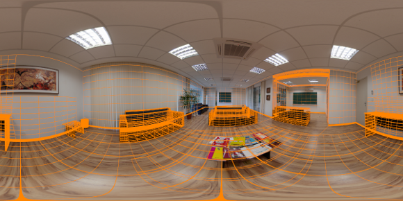
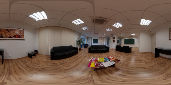
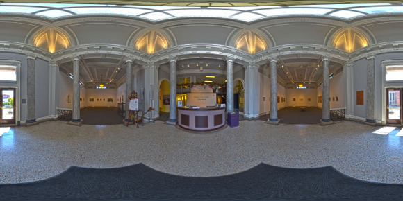
One of the most important steps on our framework is to obtain a proper representation of the environment. The environment is used for the lighting reconstruction of the scene, the calibration of the original camera device, the background plate for our renders and for the scene depth reconstruction. We settled for a industry de facto image format known as equirectangular panorama HDR images. This is a 2:1 image that encompass the captured light field. We also implemented a plugin to assist the user to rotate and accommodate the panorama in the desired position to be used in the production stage. This will be presented in more details in the next sections.
In our study we decided to use hand-modeling for the environment reconstruction. We developed a plugin for Blender, which calibrates and help this reconstruction process, guided by the captured panorama.. This is also a very flexible step, where there is plenty of freedom in which technology to adopt. For instance, the environment mesh can be obtained directly via 3d scanners. More affordable semi-automatic solutions, potentially more interesting for the independent artist, can also be reached with everyday tools like Kinect, as presented in the KinectFusion work [ 11], or with a single moving camera as described in [ 12].
We will now describe in more details the selected configuration for our experiments and show some results achieved with this approach.
In order to obtain the light field of the environment, we need to resort to capture devices. Photography cameras can be calibrated to work as a light sensor with the right techniques and post processing software. For the ambit of this project we chose to work with semi-professional photographic equipment, considering this a good trade-off between consumer cameras and full professional devices. We used Debevec’s method to produce HDR maps from bracketed pictures [ 5]. In total we took 9 pictures per camera orientation with the total of 7 different orientations to obtain the total of a  field of view from the camera point of view. The HDR stacks were then stitched together to produce an equirectangular panorama. For test our ideas we used a Nikon DX2S with a Nikon DX10.5mm fisheye lens, and a Manfrotto Pano head. For the HDR assembling we used Luminance HDR and for the stitching we used Hugin, both open source projects freely available in the Internet.
We based our panorama capturing on the study presented by Kuliyev [ 13] which presents different techniques, not discussed in the current project. Additionally, there is equipment in the market specially target for the movie making industry, not discussed in Kuliyev’s work. Expensive all-in-one solutions are used in Hollywood for capturing the environment light field and geometry (e.g., point clouding). For the purposes of this project we aimed at more affordable solutions within our reach and more accessible to a broader audience.
For future projects we consider the possibility of blending panorama video and panorama captured photography. Our approach with some considerations is as follows:
A common solution for light field capturing - mirror ball pictures - was developed to be used as reflection map and lighting [ 5]. However, when it comes to background plates, our earlier tests showed that a mirror ball picture lacks in quality, resolution and field of view. Therefore, in order to maximize the resolution of the captured light field we opted to take multiple photographies to assemble in the panorama.
To use multiple pictures to represent the environment is a common technique in photography and computational visioning. For rendered images, when a full ray tracer system is not available (specially aggravating for real-time applications) 6 pictures generated with a  frustum camera oriented towards a cube are sufficient to recreate the environment with a good trade-off between render size and pixel distortion [ 8].
We chose a fisheye lens (Nikon 10.5 mm) to increase the field of view per picture and minimize the number of required shots. We used 7 pictures in total, including the north and south pole (see figure 1).
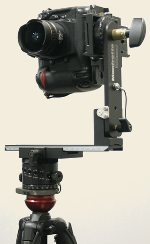
(a) Manfrotto Pano Head, Nikon DX2S camera and Nikon 10.5mm fisheye lens.
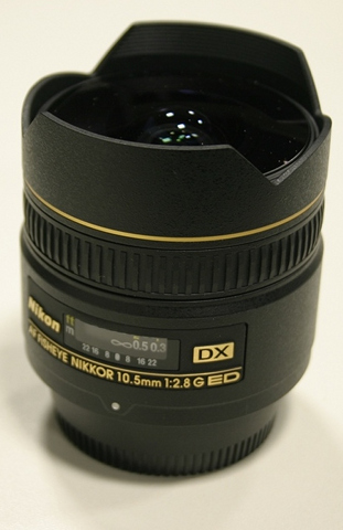
(b) Nikon 10.5mm fisheye lens.
(c) For Nikon 10.5mm: 5 photos around z-axis, 1 zenith photo and 1 nadir photo
The south pole is known for its penguins and panorama stitching problems. Many artists consider the capture of the nadir optional, given that the tripod occludes part of the environment in that direction. In fact this can be solved by the strategical placement of synthetic elements during the environment modeling reconstruction (see 6.3). To produce a complete capture of the environment we took the nadir picture without the tripod - hand-helding the camera. This can introduce anomalies and imprecisions in the panorama stitching.
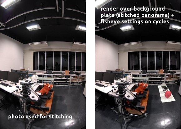
To minimize this problem, we masked out the nadir photo to contain only the missing pixels from the other shots. To give a better estimative on what to mask we stitched a panorama without the south pole, and created a virtual fisheye lens to emulate the DX2S + 10.5mm lens. The fisheye lens distortion can be calculated with the equisolid fisheye equation (1):
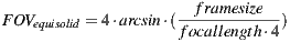 | (1) |
In the figure 2 you can see the comparison between a fisheye image taken from the camera and a fisheye render captured from the spherical panorama with the virtual lens described above. This implementation was done in Cycles, a full ray tracer renderer of Blender.
An equirectangular panorama is a discretization of a sphere in the planar space of the image. As such, there is an implicit but often misleading orientation of the representative space. The top and bottom part of the images represent the poles of the sphere. The discretized sphere, however is not necessarily aligned with the real world directions. In other words, the north pole of the sphere/image may not be pointing to the world’s zenith.
A second issue is the scale of the parametric space. The space represented in the equirectangular panorama is normalized around the camera point of view. In order to reconstruct the three-dimensional space, one needs to anchor one point in the represented space where the distance is known. For pictures not generated under controlled conditions, it can be hard to estimate the correct scale. This is not a problem as far as reconstruction of the environment goes. Nonetheless a high discrepancy in the scale of the scene should be considered for physic simulations, real world based lighting and artificial elements introduced with their real world scale in the scene.
The decision on introducing a calibration step was also to add more freedom to the capturing and obtaining of the panorama maps. The system can handle images with wavy horizons just as good as with pole oriented/aligned images.
Extra advantages of a calibration system:
- Allow to move important sampling regions off the poles.
- Less concern on tripod alignment for picture capturing.
- It works with panoramas obtained from the Internet.
- Optimal aligned axis for the world reconstruction.
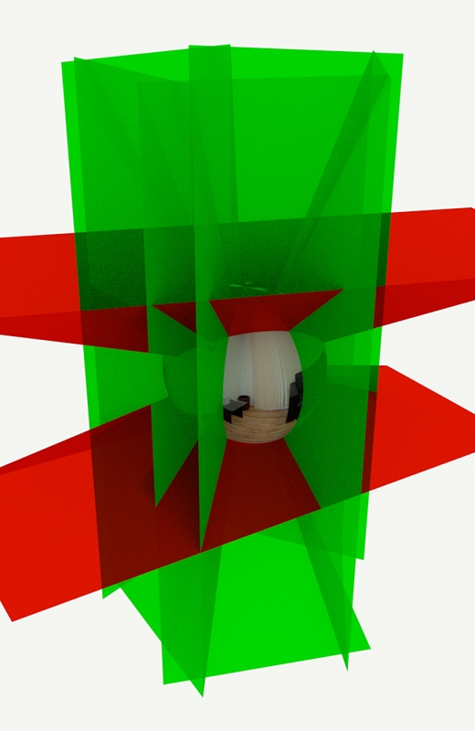
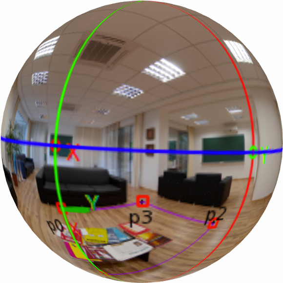
In order to determine the horizontal alignment of a panorama we chose to locate the horizon through user input on known elements. We start off by opening the panorama in its image space (mapped in a ratio of 2:1) and have the user to select 4 points  ,
,  ,
,  and
and  that represent the corners of a rectangular shape in the world space that is placed on the floor (see figure 3).
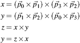
The selected points define vectors whose cross products determine the x and y axis of the horizontal plane. The cross product of x and y determines the z axis (connecting the south and the north poles). That should be enough to determine the global orientation of the image, but the manual input introduces human error to the calculation of the x and y axis. Instead of using the inputed data directly, we recalculate the y axis as the cross product of the z and the x axis in order to obtain an orthonormal basis.
To assure the result is satisfactory we re-project the horizon line and the axis in the image to provide visual feedback for user fine tuning of the calibration rectangle.
The rectangle chosen for the calibration defines the world axis and the floor plane alignment. This helps the stages of reconstruction of the existent world and the 3d modeling of new elements.

 (horizon),
  and
and  slice planes respectively. Down: Spherical representation of the panorama with the axis.
Once the orientation of the map is calculated we can project the selected rectangle onto the 3d world floor. We need, however, to gather more data - as the orientation alone is not sufficient. In fact any arbitrary positive non-zero value for the camera height will produce a different (scaled) reconstruction of the original geometry in the 3d world. For example, if the supposed original camera position is estimated higher than the position the tripod had when the pictures were taken, the reconstructed rectangle will be bigger than its original counterpart.
We have a dual system with the rectangle dimensions and the camera height. Thus we leave to the user to decide which one is the most accurate data available - the camera height or the rectangle dimensions. The rectangle dimensions are not used in the further reconstruction operations though. Instead we always calculate the camera height for the given input parameter (width or height) and use it to calculate the other rectangle side as well (height or width, respectively).
There are other possible calibration systems that were considered for future implementations. In cases where no rectangle is easily recognized, the orientation plane can be defined by independent converging axis. In architecture environments it is common to have easy to recognize features (window edges, ceiling-wall bound) to use as guides for the camera calibration.
The adopted solution is a plane-centric workflow. The calibration rectangle does not need to be on the ground. It can just as well be part of a wall or the ceiling. In our production set we had more elements to use as reference keys on the floor, thus the preference on the implementation. We intend for future projects to explore the flexibility of this system. Nonetheless this is also the reason why the environment is reconstructed from the ground up, as described in the 6 section.
6 Environment Mesh Construction
There are different reasons for the environment to be modeled. With the full reconstruction of the captured space in the panorama we can move the camera freely around and have reflexive objects to bounce the light with the correct perspective. Nevertheless, the equirectangular image is not a direct 3d map of the environment. The panorama is one of different possible parameterizations of the sphere. It lacks information to re-project the space beyond the two dimensions of the sphere surface. If we can estimate the depth of the image pixels we can reconstruct the original represented space. Therefore we can render more complex light interactions such as glossy reflections and accurate shadow orientation.
The environment meshes serve multiple purposes in our work: (a) In the rendering stage, the environment is used to compute the light position in world space for the reflection rays (see section 7.4); (b) The scene depth needs to be calculated and stored with the HDR needed by the render integrator to resolve visibility tests (see sections 7.1 and 7.3); (c) Part of the modeled environment serves as support surfaces for the shadow and reflection rendering of the synthetic elements in the assembled panorama (see section 7.2); (d) Modeled elements can be transformed while keeping their reference to how they map to the original environment to produce effects such as environment deformation and conformation to the synthetic elements (see section 6.4); (e) Finally, in the artistic production it is helpful to have structural elements for the physic animation/simulations and for visual occlusion of the synthetic elements.
There are different devices and techniques to obtain the environment mesh. The most advanced method involves depth cameras to generated point clouds to be remapped into the capture photography. This method brings a lot of precision and speed improvements to the pipeline. Those are essential features for feature-length movies that require multiple environments to be captured for a production. Another method is to capture different panoramas from similar positions, and to use a parallax-based reconstruction algorithm. The downside of this method is that it requires at least two panoramas per scene and it fails if the main captured area has no distinguished features that can be tracked.
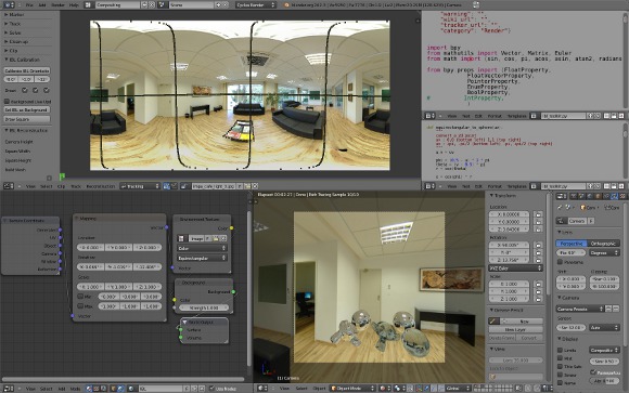
The present framework will focus on a more accessible method, which requires no special capture device or algorithm. This approach is at the same time economic and didactic. Regardless of the method adopted, it is important to understand the fundamentals of mesh reconstruction in a perspective captured environment. The scene here is reconstructed in parts. Due to the implications of the implemented calibration system, the floor is the most known region. Therefore we start modeling the object projections on the floor plane. Figure 4 shows our Blender plug-in for calibrate the panorama and modeling the environment mesh.
A system with the floor region defined in the image space and extra structuring points helps to build basic geometric elements. Two points can be used to define the corners of a square. Three points can delimitate the perimeter of a circle or define a side and the height of a rectangle.
The making of a square by its corners is a problem of vectorial math in the reconstructed 3d space. It is convenient for the 3d artist to have a canonical square defined in the local space, while determining the square size, location and rotation in the world space. Thus we use the two selected points of the image to determine the length of the square diagonal which will be used to assign the square world scale.
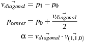
The canonical formula of the circle is defined by its center and its radius. Only in few cases you will have the center visible in the panorama though. Instead we implemented a circle defined by three points of the circumference. Even if the circle is partially occluded this method can be successfully applied.
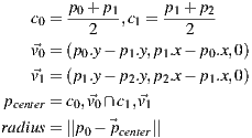
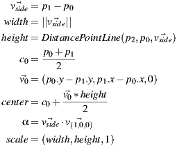
Objects that have a parallelogram geometry (for example table feet, chests, boxes) can be rebuild with a rectangular base projected on the floor. Unless their material is transparent, or only structural (for example, wires), they will have at least one of their corners occluded by its own three-dimensional body. In this case three points will have to be used to reconstruct the rectangular base.
In the pure mathematical sense, three points can define a rectangle in different ways. For instance, if they define three corners the fourth vertex can be inferred from the angles defined between the existent vertices. However, it is hard to rely on user input to precisely reconstruct the right angle intrinsic of the rectangular shape. Thus we have the user defining one of the sides of the rectangle through the two first points and setting the height with the third point. This way, even if the point does not produce a perfect right angle when projected on the floor with the defined rectangle side we can use it to calculate the distance between the opposite sides of the rectangle and ensure a perfect reconstruction of the shape.
The final shape is built in world space with the scale, orientation and position defined by the formula above. In the local space we preserve a square geometry of unitary dimensions to help the artist to adjust the real size of the geometry by directly setting its scale.
Any other simplex can be traced to outline the floor boundary or the projection of other scene elements on the floor. The points selected in the panorama image are projected to the 3d world using the camera height the same way we do for the other geometry shapes.
To rebuild elements that are not contained on the ground we needed a way to edit the meshes while looking at their projection in the panorama image. Traditionally, this is done using individual pictures taken of fractions of the set and used as background plates [ 1]. The same mapping used during render for the background plate needs to be replicated in the 3d viewport of the modeling software. In the end the environment image is mapped spherically as a background element, allowing it to be explored with a virtual camera with regular frustum (fov  ) common in any 3d software.
The implementation prioritized a non-intrusive approach in the software to ensure it can be replicated regardless of the suite chosen by the studio/artist. After every 3d view rendering loop we capture the color (with the alpha) buffer and run a GLSL screen shader with the inverse of the projection modelview matrix, the color buffers and the panorama image as uniforms. There are two reasons to pass the matrix as uniform: (a) we used the classic GLSL screen shader implementation [ 14] which re-set the projection and modelview matrices in order to draw a rectangle in the whole canvas so the shader program can run as a fragment shader on it. The matrices are then rescued before the view is setup, and the inverse matrix is calculated in CPU; (b) We need to account for the orientation of the world calculated when the panorama is calibrated (see section 5.1).

The shader performs a transformation from the canvas space to the panorama image space and uses the alpha from the buffer to determine where to draw the panorama. If the alpha channel is not present in the viewport, the depth buffer can be used. The background texture coordinate is calculated with a routine  where world is obtained with a GLSL implementation of glUnproject using the Model View Projection matrix uniform to convert the view space coordinates into the world space.
uniform sampler2D color_buffer;
uniform sampler2D texture_buffer;
uniform mat4 projectionmodelviewinverse;
#define PI 3.14159265
vec3 glUnprojectGL(vec2 coords)
{
float u = coords.s * 2.0 - 1.0;
float v = coords.t * 2.0 - 1.0;
vec4 view = vec4(u, v, 1.0, 1.0);
vec4 world = projectionmodelviewinverse * vec4(view.x, view.y, -view.z, 1.0);
return vec3(world[0] * world[3], world[1] * world[3], world[2] * world[3]);
}
vec2 equirectangular(vec3 vert)
{
float theta = asin(vert.z);
float phi = atan(vert.x, vert.y);
float u = 0.5 * (phi / PI) + 0.25;
float v = 0.5 + theta/PI;
return vec2(u,v);
}
void main(void)
{
vec2 coords = gl_TexCoord[0].st;
vec4 foreground = texture2D(color_buffer, coords);
vec3 world = glUnprojectGL(coords);
vec4 background = texture2D(texture_buffer, equirectangular(normalize(world)));
gl_FragColor = mix(background, foreground, foreground.a);
}
The background is consistent even for different frustum lens and camera orientations. This technique frees the artist to create entirely in the 3d space without the troubles of the image/panorama space. For a perfect mapping it is important to use an image with no mipmaps or to use the GLSL routine to specify which mipmap level to access ( ).
).
6.3 Removal of Environment Elements
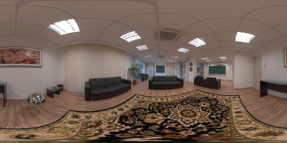
Modeling can be quite time consuming and a very daunting task. Some elements present in the environment may be undesired in the final composition. One example is the table in the middle of the scene showed along this paper. We inserted a synthetic carpet in the scene in a way that it completely overlays the table in the panorama image space.
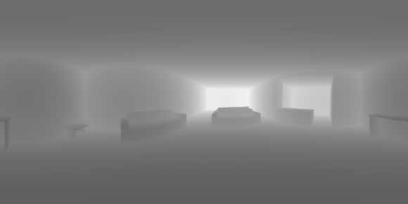
In the figure 5 you can see the carpet rendered in details. Also notice that we do not need the table to be modeled for the depth map (see the center figure). In the end if the object does not exist in the depth or the light parts of the map, it is as if it was never there. The same technique can be used to handle missing nadir capture (see section 4.2).
6.4 Environment Coordinates Projection
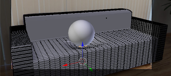
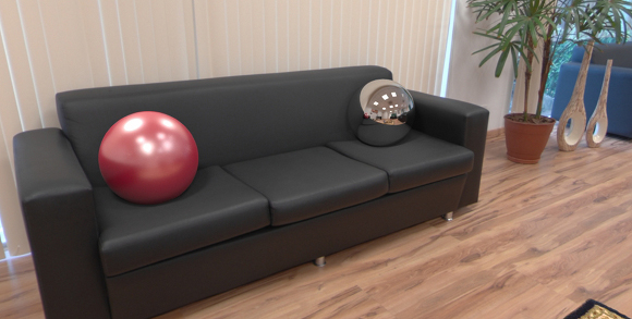
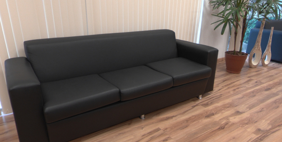
We are using a method to transform the environment by deforming the support mesh created using the image as reference. Once the artist is satisfied with the accuracy of the mesh of the object to be transformed, she can store the panorama image space coordinates (UV) of each vertex in the mesh itself. From that point on, any changes in the vertices position can be performed as if affecting the original environment elements. For example, we can simulate a heavy ball (synthetic element) bouncing on a couch (environment element) and animate the deformation of the couch pillows to accommodate the weight of the ball. In the figure 6 you can see the couch modeled from the background image and the mesh deformation under the synthesized sphere.
The renderer should be capable of using this information to always use the light information from the stored coordinates instead of the actual position of the vertices. This works similar to traditional UV unwrapping and texture mapping. In fact this can be used for simple camera mapping (using this as UV and passing a LDR version of the panorama as texture) in cases where the renderer can not be ported to support the augmented reality features implemented in the ENVPath integrator, section 7.6. This can also be used to duplicate the scene elements in new places. A painting can move from one wall to another, the floor tiling can be used to hide out a carpet present in the environment, and so on.
For the ENVPath integrator the UV alone is not enough. The vertices in the image space are represented by a direction, but we need to be able to store the original depth of the point as well. Therefore we store in a custom data layer not the UV/direction, but a 3-float vector with the original position of each vertex. We take advantage that both Blender internal file format and the renderer native mesh format can handle custom data. The renderer supports ply as mesh format, so we extended it with property float wx, property float wy and property float wz. The data needs to be stored in the world space (in oppose to the local space) to allow for the mesh to suffer transformations at the object level, not only at the mesh.
6.5 Modeling More than Meets the Eye
Even with a static camera we may need to know more information from the scene than what was captured originally in the panorama. For example, if a reflexive sphere is placed inside an open box you expect to see the reflection of the interior of the box in the sphere even if it was not visible from the camera point of view (and consequently is not visible in the pictures taken). Another case is to perform camera traveling in the 3d world. A new camera position can potentially reveal surfaces that were occluded before, and for them there is no information present in the panorama.
There are three solutions we considered for this problem: (1) If the occluded element is not relevant for the narrative it can simply be ignored completely as if it was never present in the real world (for example, an object lost underneath the sofa, invisible from the camera position); (2) In other cases the artist needs to map a texture to the modeled element and create a material as she would in a normal rendering pipeline. (3) A mesh with the environment coordinate stored can be used to fill some gaps (see section 6.4).
The main problem in the traditional method for rendering based in environment maps is that all light scattering computations are performed using the environment map as a set of directional lights. This approach has the drawback that the environment map must be captured in the position where the synthetic objects are to be inserted into the real scene, as did Devebec in his work [ 6]. If we need to introduce several objects in different positions of the scene, we will have problems with the positions of the shadows and reflections from objects in the final render (see figure 14). In addition to the above problems, if the map resolution is poor, we also have to get the background of the scene separately through photographs or video, and this makes the panoramic rendering more difficult.
The proposed framework allows us to model and synthesize a full panoramic scene using a single large resolution environment map as input. This map is used for rendering the background, apply textures and model the environment geometry to keep photo-realistic light scattering effects in the final augmented panoramic scene to be rendered.
The rendering integrator, ENVPath, used in this production framework is a modified path tracing algorithm, but with changes in implementation due to new features explored here. It was developed during the course of this research but its specific details are outside the scope of this paper. We will review here some key ideas of the rendering process to help the reader understanding the decisions taken in the production process. The ENVPath integrator is fully described in [ 15].
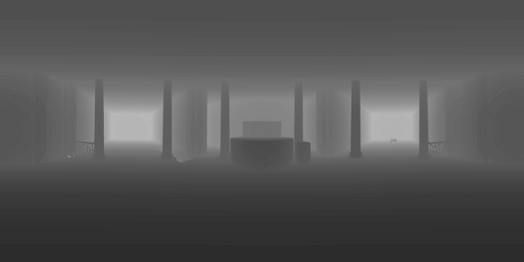
7.1 Light-depth Environment Maps
In this paper we introduce a new type of space representation, the light-depth environment map. This map contains both radiance and the spatial displacement (i.e., depth) of the environment light. The traditional approach for an environment map is to take it as a set of infinite-distant or directional lights. In this new approach the map gives information about the geometry of the environment, so we can consider it as a set of point lights instead of directional lights. This second approach results in a more powerful tool for rendering purposes, because the most common environment maps have their lights originally in a finite distance from the camera, such as an indoor environment map. With the depth we can reconstruct their original location and afford more complex and accurate lighting and reflection computations. This enhanced map is no longer a map of directional lights but a conglomeration of lights points.
A light-depth environment map can be built from an HDR environment map adding the depth channel, as shown in figure 7. The depth channel can be obtained by a special render from the reconstructed environment meshes or also by scanning of the environment or other techniques.
For the following mathematic notations, a pixel sample from the light-depth environment map is denoted by  , where
  is the direction of the sample light in the map and the scalar value
  denotes the distance from the light sample to the light space origin. The position for the light sample in the light space is given by the point
  .
.
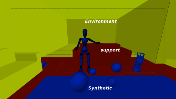
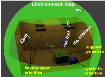
7.2 Primitives: Synthetic, Support and Environment Surfaces
The rendering integrator used for this work needs a special classification for the different scene primitives. Each primitive category defines different light scattering contributions and visibility tests. Basically we classify the primitives into three types as shown in figure 8.
- Synthetic primitives: the objects that are new to the scene. They do not exist in the original environment. Their light scattering computation does not differ from a traditional path tracer algorithm.
- Support primitives: surfaces present in the original environment that needs to receive shadows and reflections from the synthetic primitives. Their light scattering computation is not trivial, because it needs to converge to the original lighting.
- Environment primitives: all the surfaces of the original environment that need to be taken into account for the reflection and shadow computation for the other primitive types. They do not require any light scattering computation, because their color is computed directly from the light-depth environment map.
The level of detail of the environment reconstruction (see section 6) will depend on how you need the final render to be. For example, in a scene with no objects with glossy reflections, the environment mesh can be simplified to define only the main features that contribute with the lighting of the scene (e.g., windows and ceiling lamps) and a bounding box. Every ray starting at the light origin in world space must intersect with some primitive. Since our primary goal is to render a full panorama image, we need to make sure the light field has the depth of all the rays. Thus it is important to model the environment mesh around all the scene without leaving holes/gaps.
For every camera ray that intersects with the scene at a point  on a surface, the integrator takes a light sample
  by importance from the depth-light map to compute the direct light contribution for point
  . Next, the renderer performs a visibility test to determine if the sampled light is visible or not from the point
  .
.
In the traditional rendering scheme, that uses environment maps as directional lights, the visibility test is computed for the ray  , with origin in
  and direction
  with
with  in world space. This approach introduces several errors when the object is far away from the point where the light map was captured. Note that all the shadows will have the same orientation, given that only the direction of the light sources is considered.
 used by the directional approach is not occluded, so the light
  contributes for the scattering account of point
  . The ray
  used by our light-positional approach is occluded by a synthetic object, thus it gets the correct world-based estimation.
9(b): Reflection account. The ray
 intersects the scene at point
  , over the environment mesh. The radiance of
  is stored at
  direction in the light-depth map. The correct reflection value is given by
  , instead the ray
  used in the traditional approach.
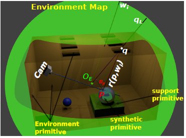
Our rendering algorithm works differently. Thanks to the light-depth environment map properties, the visibility test uses the light sample world position and not only its direction.
The new visibility test use the direction  of the light sample and multiply it by their depth value
  obtaining the point
  in the coordinate system of the light. The point
  is transformed to world space to obtain
 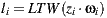 . Thus the calculation of visibility is made for the ray
  , with origin
  and direction
  as shown in figure 9(a).
Given a point  on a surface, the integrator takes a direction
  by sampling the surface BRDF (Bidirectional Reflectance Distribution Function) to add reflection contributions to the point
  . To do this, we compute the scene intersection of the ray
  with origin
  and direction
  . Note that the intersection exists because the environment was completely modeled around the world. If the intersection point
  is on a synthetic or support surface its contribution must to be added to reflection account. Otherwise, if the intersection is with an environment mesh, we transform
  from world space to light space by computing
  . Finally the contribution given by the direction
  in the environment map is added to the reflection account. The figure 9(b) illustrates this proposal.
7.5 Environment Texture Coordinates
Environment texture coordinates was implemented to support rendering effect such as the deformation in the original environment by the interaction with synthetic objects. Another application is to copy a texture from one environment region to another. This can be a powerful tool for texturing support meshes on regions where do you do not know the color directly by the environment because they are occluded by other support object. In figure 10 we show the power of this tool to apply deformations on support objects when they interact with synthetic objects.
7.6 ENVPath Integrator: Path Tracing for Light-Depth Environment Maps
We use an implementation of the path tracing algorithm that solves the light equation constructing the path incrementally, starting from the vertex at the camera  . At each vertex
  , the BSDF is sampled to generate a new direction; the next vertex
  is found by tracing a ray from
  in the sampled direction and finding the closest intersection.
For each vertex  with
with  we compute the radiance scattering at point
  along the
  direction. The scattering contribution for
  is computed estimating the direct lighting integral with an appropriate Monte Carlo estimator for the primitive type (synthetic, support or environment surface) of the geometry the vertex
  belongs to.
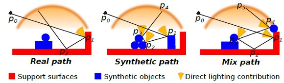
A path 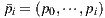 can be classified according the nature of its vertices as
- Real path: the vertices
 ,
,  are on support surfaces.
 - Synthetic path: the vertices
 ,
,  are on synthetic objects surfaces.
 - Mixed path: some vertices are on synthetic objects and others on support surfaces.
There is no need to compute any of the real paths for the light. Their contribution is already stored in the original environment map. However, since part of the local scene was modeled (and potentially modified), we need to re-render it for these elements. The computed radiance needs to match the captured value from the environment. We do this by aggregating the radiance of all real paths with same vertex  as direct illumination, discarding the need of considering the light contribution of the subsequent vertices of the paths.
 that contributes with the illumination accounts. Vertex without the yellow cones do not contributes for the for the illumination accounts.
The synthetic and mixed light paths are computed in a similar way, taking the individual path vertex light contributions for every vertex of the light path. The difference between them is in the Monte Carlo estimate applied in each case. In the figure (11) it is possible to see the different light path types and the computations that happens on the corresponding path vertices.
Because we are using an incremental path construction technique, it is impossible to know the kind of path we have before we are done with it. Thus the classification above is only theoretical.
For implementation purposes during the incremental path construction we only need to know if the partial path ( ) contains some synthetic vertices or not. This allows us to decide what Monte Carlo estimator we need to use. To do this, we use a boolean variable
  (path type) that has a false value if the partial path does not have synthetic vertices and true otherwise.
The rendering time of the proposed algorithm is equivalent as what we can obtain with other physically based rendering algorithm using a scene with the same mesh complexity. Part of the merit of this, is that this is an one-pass solution. There is no need for multiple composition passes. And the rendering solution converges to the final results without ’adjustments’ loops been required like the original Debevec’s technique [ 6].
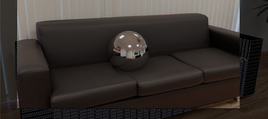
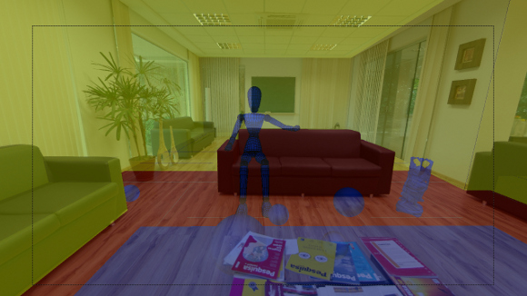
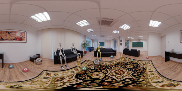
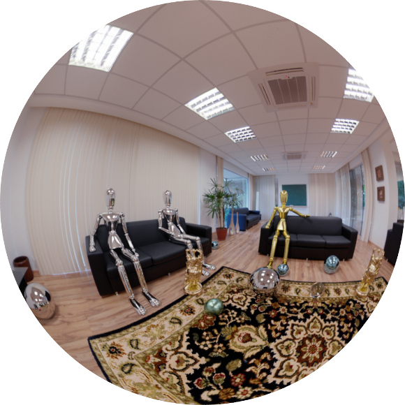
As explained during the paper, the core aspect of this process is to is to mix rendered and captured full panorama images. More specifically the integration of a captured environment and synthetic objects. In the figures 12 and 13 you can see the synthetic elements integrated with the original panorama. In each case the lighting and shadows of the synthetic elements over the original environment are computed using the light-depth map.
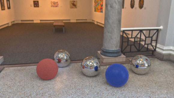
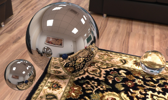
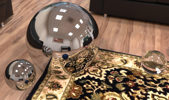
The mirror ball reflection calculation can be seen in more details in the figure 14. This is a comparison between the traditional direction map method and our light-depth map solution. The spheres and the carpet are synthetic and are rendered alike with both methods. But the presence of the original environment meshes makes the reflection to be a continuous between the synthetic (e.g., carpet) and the environment (e.g., wood floor).
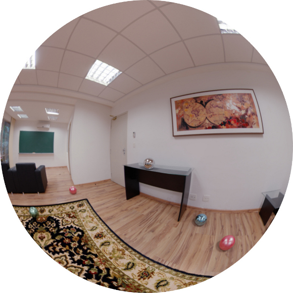
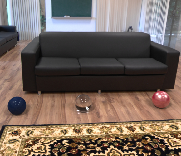
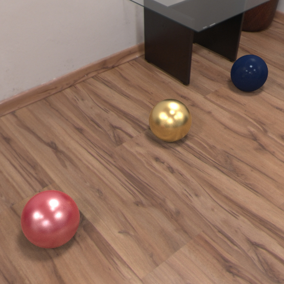
The proper calibration of the scene and the correct shadows help the natural feeling of belonging for the synthetic elements in the scene. In the figure 15 you can see the spheres and the carpet inserted in the scene. The details are shown in a non panoramic frustum to showcase the correct perspective when seen in a conventional display.
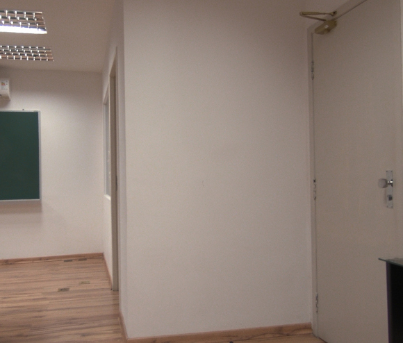
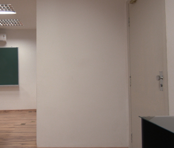
Finally, we explored camera traveling for a few of our shots. In the figure 16 you can see part of the scene rendered from two different camera positions. The result is satisfactory as long as the support environment is properly modeled. For slight camera shifts this is not even a problem.
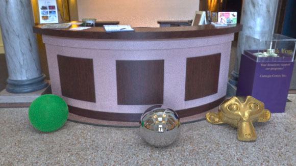
To ensure this frameworks was flexible enough, we explored this pipeline using a panorama captured by a third party. From there we reconstructed the depth, added synthetic elements and produced some images. The satisfying renders are on figure 12.
We have presented a general framework for adding new objects to full panoramic scenes based on illumination captured from real world and reconstructed depth. To attest the feasibility of the proposed framework we applied it into the production of realistic immersive scenes for panoramic and conventional displays.
A key point of our method, until now unexplored to those means, is the use of the light positions in the environment map instead of the directional approach, to get the correct shadows and reflections effects for all the synthetic objects along the scene.
Among the possible improvements, we are interested on studying techniques to recover the light positions for assembling the light-depth environment map and semi-automatic environment mesh construction for the cases where we can capture a point cloud of the environment geometry.
A shortcoming of this solution is the lack of freedom in the camera movement within the rebuilt scene. This is a limitation of using a single captured panorama. Even without moving the camera there are blind spots due to objects being occluded from the camera point of view. This is more evident when the missing information was supposed to be reflected by one of the synthetic objects.
As a further development of this project we want to explore the capture of multiple panoramas. We are working on determining an optimal number of captures to fully represent a scene. This will allow more complex camera traveling without compromising too much of the performance. Additionally, this prevents the abuse of copying the environment texture to complete unknown environment elements. The environment texture copy (and paste) solution is better fit for applying soft deformations on the environment elements.
Finally, we were quite pleased with the results of this framework to produce content for conventional displays. Camera panning and traveling works regardless of the camera frustum and field of view. For non-panoramic frustums camera, zooming can also be used to deliver the essential camera toolset for traditional filmmaking.
[1] A. R. Zang and L. Velho, “Um framework para renderizações foto-realistas de cenas com realidade aumentada,” in XXXVII Latin American Conference of Informatics (CLEI), Quito, 2011.
[2] ——, “Arluxrender project,” in http://www.impa.br/ zang/arlux. Visgraf, 2011.
[3] G. S. Miller and C. R. Hoffmanm, “Illumination and reflection maps: Simulated objects in simulated and real environments,” in Curse Notes for Advanced Computer Graphics Animation. SIGGRAPH, 1984.
[4] L. Williams, “Pyramidal parametrics,” in Proceedings of the 10th annual conference on Computer graphics and interactive techniques. ACM-SIGGRAPH, 1983, pp. vol 17(3), pp. 1–11, ISBN:0–89 791–109–1.
[5] P. E. Debevec and J. Malik, “Recovering high dynamic range radiance maps from photographs.” SIGGRAPH, 1997, pp. pp. 369–378.
[6] P. E. Debevec, “Rendering synthetic objects into real scenes: Bridging traditional and image-based graphics with global illumination and high dynamic range photography.” SIGGRAPH, 1998, pp. pp. 189–198.
[7] D. F. K. Karsch, V. Hedau and D. Hoiem, “Rendering synthetic objects into legacy photographs,” in Proceedings of the 2011 SIGGRAPH Asia Conference. pp. 157:1–157:12: ACM, New York, NY, USA, 2011.
[8] P. D. Bourke and D. Q. Felinto, “Blender and immersive gaming in a hemispherical dome,” in GSTF International Journal on Computing (JoC), 2010, pp. Vol. 1, No. 1, ISSN: 2010–2283.
[9] D. Felinto and M. Pan, Game Development with Blender. Cengage Learning, 1st ed., 2013.
[10] D. Q. Felinto, “Domos imersivos em arquitetura,” in Bachelor thesis at the Escola de Arquitetura e Urbanismo. Niterói: Universidade Federal Fluminense, 2010.
[11] R. A. Newcombe, A. J. Davison, S. Izadi, P. Kohli, O. Hilliges, J. Shotton, D. Molyneaux, S. Hodges, D. Kim, and A. Fitzgibbon, “Kinectfusion: Real-time dense surface mapping and tracking.”
[12] R. A. Newcombe and A. J. Davison, “Live dense reconstruction with a single moving camera,” in IEEE Conference on Computer Vision and pattern Recognition, 2010.
[13] P. Kuliyev, “High dynamic range imaging for computer imagery applications - a comparison of acquisition techniques,” in Bachelor thesis at the Department of Imaging Sciences and Media Technology. Cologne: University of Applied Sciences, 2009.
[14] R. J. Rost and B. Licea-Kane, OpenGL Shading Language. The Khronos Group, 3rd ed., 2010.
[15] D. F. A. Zang and L. Velho, “Rendering synthetic objects into full panoramic scenes using light-depth maps,” Visgraf Technical Report (submitted to GRAPP 2013), Tech. Rep.

