


Services on Demand
Journal

Article
 Spanish (pdf)
 Article in xml format
 Article references
Related links
Share

 Permalink
CLEI Electronic Journal
On-line version ISSN 0717-5000
CLEIej vol.16 no.1 Montevideo Apr. 2013
Departamento de Sistemas de Computação,
Instituto de Ciências Matemáticas e de Computação,
Universidade de São Paulo,
São Carlos, Brazil, PO Box 668, 13560-970
{steiner, masiero}@icmc.usp.br
Rodrigo Bonifácio
Departamento de Ciência da Computação,
Instituto de Ciências Exatas,
Universidade de Brasília,
Brasília, Brazil, PO Box 4466, 70910-900
rbonifacio@cic.unb.br
Abstract
Unmanned Aerial Vehicles (UAV) are vehicles that fly without a pilot and are able to execute different types of missions, such as surveillance, topographical data collection, and environment monitoring. This motivates some degree of variability in the controlling software of UAV – usually specified using Simulink models –, even though it is also possible to reuse software in this domain using systematic approaches such as Software Product Lines (SPLs). In this paper we present a catalog of patterns to represent variable features in Simulink and show how to construct a simple software product line for an UAV. We also show mechanisms and an infrastructure for configuring Simulink assets, using two tools to manage variabilities: Pure::variants and Hephaestus. These tools are also compared according to a set of characteristics.
Spanish Abstract:
Los vehículos aéreos no tripulados- Unmanned Aerial Vehicles (UAV) son vehículos que vuelan sin piloto y son capaces de ejecutar diferentes misiones. Esto motiva un grado de variabilidad en el software de control, aunque es posible reusar software en este dominio utilizando enfoques sistemáticos como el de Software Product Lines (SPLs). En este trabajo presentamos un catálogo de patrones para representar aspectos diferentes de Simulink y mostramos como construir una línea de producto de software para un UAV.
Keywords: Unmanned Aerial Vehicles, Simulink Models, Software Product Lines, Pure::variants, Hephaestus.
Portuguese Keywords: Linha de Produtos de Software, Veículos Aéreos Nao Tripulados, Simulink
Received 2012-07-09, Revised 2012-12-13, Accepted 2012-12-13
The approach of software product line (SPL) is ideal for software domains where the objective is to develop a set of products that have common characteristics and variable parts. Using this approach it is possible to develop systems with much less time and effort compared to traditional development approaches (focusing on a single system). A software domain that has these characteristics is the one related to the control of Unmanned Aerial Vehicles (UAV), which includes an autopilot.
The Software Product Line (SPL) approach has been successfully used in the development of embedded systems. It looks for commonalities and variabilities within a family of products and maintains a set of core assets to leverage reuse. We have already explored the development of a SPL for UAVs using an approach called ProLiCES (1). In the implementation phase, contrarily to many other proposals in this domain, we have used a model-based approach that uses Simulink models to generate C code.
Nevertheless, there are just a few works (2, 3) that investigate how to model and manage variabilities in this environment. Thus, in this paper we show a catalog of patterns to model variabilities in Simulink and a simple SPL that has been developed to test our approach. Here we also explain how to manage configurability of SPL assets modeled in Simulink, considering two alternative product derivation tools tailored to manage variability in SPL Simulink models. This paper also shows how these tools have been used to configure variabilities of a Simulink model of a UAV. Furthermore, a comparison of the main features, benefits and drawbacks of each tool is presented.
This paper is organized as follows: Section 2 introduces some related work, considering SPLs for Unmanned Aerial Vehicles, modeling SPL variability in Simulink models, and tool support for modeling SPL variabilities in Simulink models. Section 3 presents one of the contributions of this paper, which is an extended approach for modeling SPL variabilities in Simulink models. Then, in Section 4 we model the variabilities of Tiriba (a small-sized UAV) using our approach. In order to do that, we first customized two existing tools (Pure::Variants and Hephaestus) for product derivation, accordingly the requirements of our approach. Section 4.1 and Section 4.2 detail the customization of such a tools. In Section 5 we compare the use of Pure::Variants and Hephaestus to manage SPL variability and product derivation and, finally, Section 6 presents our conclusions and some future works directions.
2.1 Software Product Lines for Unmanned Aerial Vehicles
The Software Product Line (SPL) approach aims to develop a set or family of software products within a specific domain (4). Products of a family have a common part (a reusable architecture) and variable parts that satisfy different requirements. An important SPL concept is the one of a feature, which is a functional characteristic considered relevant for both customers and developers (5, 6). Features might be mandatory, optional or alternative, and its structure and relationships are usually represented as feature diagrams.
Variability management is the activity responsible for defining, representing, exploring, implementing, and evolving the variabilities of an SPL. According to Pohl et al (7) this activity includes the following sub-activities: manage variable artifacts, support activities related to the definition of variabilities, support activities focused on resolving variability and collect, store and manage traceability information needed to accomplish those tasks.
Among the responsibilities of tools that support SPL variability management, it is also included that of generating specific products of the line. Generation of products can be accomplished using either positive or negative variability techniques. The derivation of products with negative variability starts with a template that contains the unification of all features of an SPL and changes them removing or disabling features that are not selected. Differently, in the positive approach, a specific asset relates fragments of artifacts with features of an SPL. During the product derivation, these fragments will be added or not to the product depending on the feature configuration.
There are many cases of SPL developed with success in the domain of embedded systems. A large number of companies have used the approach to develop its products, such as Siemens, Nokia, Philips and HP (4, 7). Unmanned Aerial Vehicles (UAV) is one of the different types of embedded systems that might be worthwhile to apply the SPL approach. UAV is an expression that refers to aircrafts that can fly without a pilot, or an aircraft structure and an embedded computer system which, combined with sensors, GPS, actuators and CPUs are able to fly without human intervention (8).
The UAVs have been originally designed for military applications, because they provide safe solutions at a relatively low cost for various types of missions, such as: surveillance, spying and blocking or interfering with radars. In addition to military applications these aircrafts are increasingly being used in civilian, commercial, and scientific applications such as meteorological measurements, topographic data collection, assessment of incidents of catastrophic proportions, agriculture monitoring, fishing, and environment.
Tiriba is a small-sized, electrically motorized UAV developed in partnership between the company AGX and the INCT-SEC (National Institute of Science and Technology for Critical Embedded Systems) (9, 10). Its design was created using an approach based on Simulink models from which C code is automatically generated. Simulink is an integrated development environment based on models for system’s analysis, modeling and simulation developed by Mathworks (11). It uses the infrastructure of MATLAB, which enables the modeling of linear dynamic systems, nonlinear, continuous or discrete in time. Using Simulink it is possible to design, simulate, test and generate code for many types of systems, including communication systems, control and signal processing, image and video.
Developers represent a system using Simulink models by means of blocks and the execution and communication among blocks use a synchronous time model. Simulink contains a library with various types of blocks, each one representing a different dynamic process. Besides modeling in blocks, which is called dataflow, Simulink allows interaction of its models with finite state machines (FSM) and with algorithms coded in MATLAB.
2.2 Modeling SPL Variability in Simulink Models
A few authors have discussed in the literature how to model variabilities in Simulink. Nonetheless, the negative approach seems to be preferred due to the graphical nature of Simulink modeling. Polzer et al. combine model driven techniques with rapid application development to manage variability within a sensor network (3). Using their proposed approach, the configuration process not only selects sensors and actuators based on the specific features of an SPL instance, but also tailors the micro-controller behavior according to the resulting configuration. The micro-controller behavior is specified using Simulink models, while the component variability (or parameterization is this case) is specified using a different asset (a configuration file). Using a well established practice of the SPL approach, domain engineers specify the scope of the product line using feature models (6). Finally, the product derivation is supported by the pure::variants tool and the Simulink connector (we discuss tool support for Simulink product lines in Section 2.3).
Botterweck et al. also present a product derivation process for SPL Simulink models (12), which follows a negative and transformational style (see Section 2.1). In order to derive valid Simulink models, corresponding to the union of all selected features, it is necessary to use the variability mechanisms of Simulink blocks for each feature. Therefore, optional features might be represented using enabler subsystems— in the cases where the enabler port is 0, the subsystem will be absent. Alternative features might be represented using switch blocks, which have three input gates. The output value of a switch block is either the value of the first or third gate, depending on both the configuration value of its condition and the value of the second gate. Finally, inclusive-or features might be represented using integrator blocks, which could implement different functions such as minimum and maximum. In their work, the instantiation process comprises two phases: product derivation and pruning. During product derivation, all blocks not related to the selected features must be removed from the resulting Simulink model. During the pruning phase, all invalid lines (which are not connected to a source block, target block, or both) must be removed from the resulting Simulink model, as well as the remaining variability mechanisms. All transformations lead to a valid Simulink model including only the blocks related to the selected features and the required lines.
Moreover, some approaches have been proposed to represent SPL variability in the vehicle domain, for both the automotive industry (13, 14) and UAV systems (15). For instance, Fragal et al. describe an approach for mapping SPL features to UAV Simulink models, using a negative technique for product derivation (15) that basically considers one-to-one or one-to-many mappings between features and blocks. Here we go beyond this simple kind of mapping, allowing relationships between feature expressions using propositional logic and differente components of simulink models (such as blocks and final state machines). Our approach is also guided by a set of variability patterns described in Section 3.
Nevertheless, we also follow a negative approach for product derivation, using two disctinct methods for relating the problem space (represented as feature models) and the solution space (here represented by Simulink models). In the first method (that we implement using Pure::variants) we have to instrument the underlying model with mechanisms to model the SPL features— this is an example of annotative based method (16). In the second method (that we implement using Hephaestus) we relate feature expressions to model transformations. In this case, which is an example of a compositional method (16), product derivation is fullfilled by applying the set of transformations that are related to the feature expressions satisfied by the product configuration. Both methos are respectively presented in Section 4.1 and Section 4.2.
2.3 Tool Support for Modeling SPL Variability in Simulink Models
There exist several tools for managing variability in SPLs, and Torres et al. present an assessment of some of these tools (Pure::variants, Hephaestus, GenArch, ColorIDE, and XVCL) in the context of SPL evolution (17). We decided to use Pure::variants and Hephaestus to implement the tool support for our approach, since our goal here is to investigate the use of annotative and compositional methods to manage SPL variability of UVA Simulink models. We decided to implement the annotative approach using Pure::variants because a Simulink connector was already available at the time we started this research. Our decision to use Hephaestus is that, differently from the other mentioned tools, it is primarily based on a compositional approach, where no explicit annotation is required in the underlying model. Moreover, the third author of this paper is the lead Hephaestus developer, reducing the risks to implement a Hephaestus Simulink integration.
Pure::variants is a widely used business tool for managing variabilities in product lines. Among the plugins of the tool, there is the Simulink connector, which uses an approach similar to that proposed by Dziobeck et al.(2). The management of variability with Simulink connector uses the concept of “point of change”, which encapsulates the variability information of a particular functional variant. It uses a unique identifier and also:
- A variability parameter, which describes a configuration parameter in a Simulink model that can be configured to select a functional variant.
- Mechanisms of variability, which describe how functional variants are selected in different parts of Simulink models. They guarantee that after parameters of variability are configured, only the selected variants are executed. These variability mechanisms are implemented by a set of specific blocks of Pure::variants that are exported to Simulink. Examples of blocks used as mechanisms of variability are presented in Section 2.2.
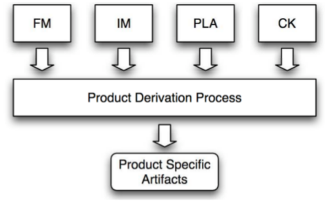
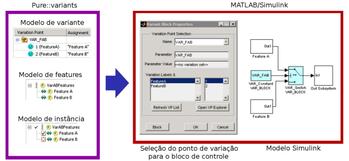
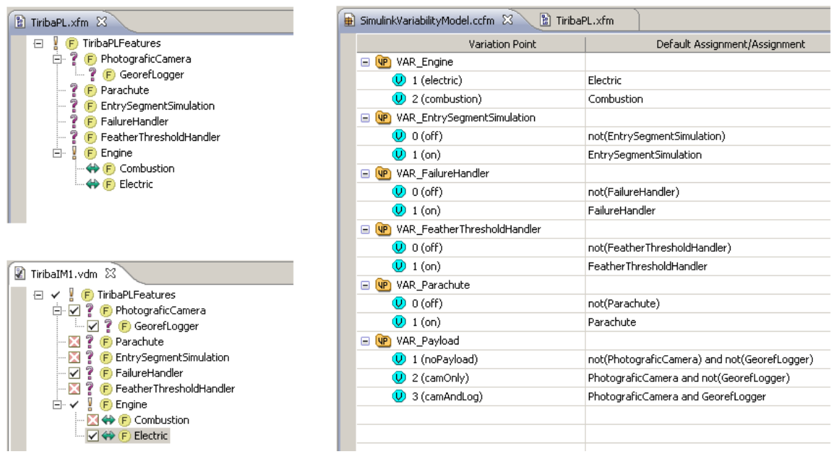
Most of the variability mechanism blocks need input signals to control their execution, thus serving for the selection of variability. The blocks responsible for these signs are called control blocks and usually control variabilities in the model using values defined by the variability parameter of their variation point. Pure::variants sets the value of the variability parameter used by the control blocks based on three main artifacts: features model, instance model (a valid configuration of features of the feature model) and variant model. The latter maps expressions of features from the feature model to values of the variability parameters, as depicted in Figure 1.
Hephaestus is a tool to generate artifacts of specific instances of SPLs. In its current version, it supports variability management of different types of assets, such as use case scenarios, source code and business processes (18). Hephaestus contains a graphical interface that allows application engineers to select artifacts and models that are input to the process of product derivation. The tool evaluates the artifacts and models and then generates artifacts for specific instances of an SPL. Figure 2 shows a high level view of Hephaestus. The input artifacts and models are: features model, instance models, product line assets, and configuration knowledge. The instance model represents the configuration of the features of a product and the configuration knowledge maps feature expressions to transformations that to be performed on the SPL assets.
Nowadays there are different representations of the configuration knowledge, the simplest of which basically maps a feature to a SPL asset. The process of deriving products used by Hephaestus starts evaluating each feature expression of the configuration knowledge from selected features of the instance model. All transformations associated to the feature expressions evaluated as true are applied to the SPL assets selected for the process; these transformations select or modify parts of the assets for the product that is being generated.
Hephaestus has been recently extended as part of this work to allow for the generation of instances of SPL products in Simulink. The configuration knowledge defined in this extension associates with each feature expression of a set pairs, each comprised by a block identifier and a transformation to be applied to that block.
Two transformations have been implemented in Hephaesuts: selectSimulink-Block, which should be linked to the block identifiers that will be selected for the instance model and clearVariabilityMechanism which should be associated to blocks that implement variability mechanisms (as we detail in the next section).
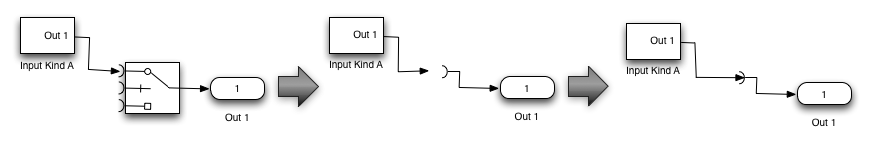
First selectSimulinkBlock transformations are executed by introducing into the instance model all blocks that are related to the selected features, as well as the connections betweem each one of these blocks. After the evaluation of all selectSimulinkBlock transformations, the transformations of the clearVariabilityMechanism are executed. In the current status of Hephaestus this transformation removes the block marked as the variability mechanism associated to it, and reconnects the block connected to its entry in the block connected to its output. An example of how this transformation can be configured and applied is shown in Figure 3: the switch block is associated to the processing clearVariabilityMechanism, and blocks A, Input Kind, and Out1 are associated with the transformations selectSimulinkBlock (having already been performed). In the figure, one can see step by step how Hephaestus applies the transformation clearVariabilityMechanism: the variability blocks are removed and the selected block connected to the input of the block used as variability mechanism is connected to its output block.
3 An Extendend Approach for Modeling Variability in Simulink Models
In order to design an SPL Simulink model, it is necessary to use a few mechanisms to model variability in different parts of the model. The main reason for that is to avoid an invalid model and to adequately bear the model variability making possible to simulate and generate SPL product specific code.
As mentioned in section 2.2, Botterweck et al. (12) introduced some mechanisms for that purpose. In their work, these mechanisms model variability of optional features and features with or-inclusive and or-exclusive relationships. In this section we extend the mechanisms proposed by Botterweck et al. showing two patterns to configure features with hierarchical or dependency relations in the dataflow part of Simulink models and two patterns to configure variability in MATLAB/Simulink finite state machines (FSM).
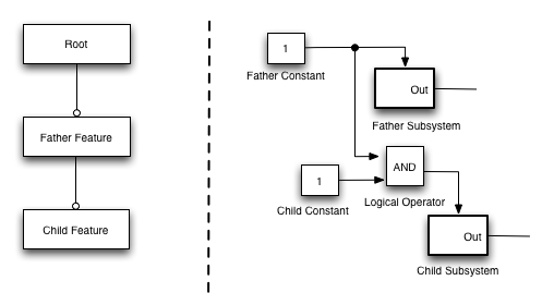
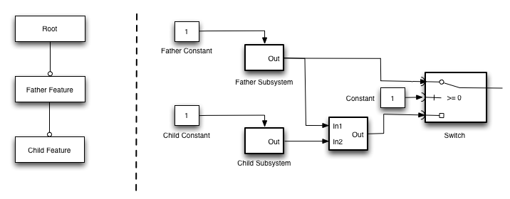
A variability mechanism for features with dependency or hierarchical relation with its functional variants encapsulated in one or more enabler subsystems is created using an AND comparator block; which is used to determine whether the input on the enabler port of the feature dependent (or child feature) enabler subsystem will be enabled or disabled. The enabler subsystem will be enabled only in the cases where both the activation value of the father and child features are true (thus the output of the AND block will also be true). If one of the activation values is false, the subsystem related to the child feature will be disabled. Figure 4 shows an example of this pattern, considering that the activation values of the features are determined by constant blocks.
In the cases where the signals of dependent features are both used in the same subsystem of a model, it is possible to use a switch block as a variability mechanism (Switch Pattern). Figure 5 shows an example, where if both features are selected, the input of the control port of the switch block must be set to get the output of the block that uses the signals of the father and child features. Otherwise, the input of the control port must be set to get the output of the father’s block.
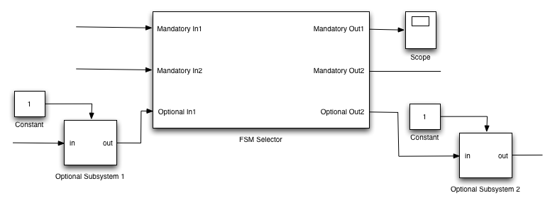
The interaction with FSMs is a common property of many Simulink models. Thereby, besides the variability in the dataflow part of the models (as explained before), an SPL Simulink model must also considers FSM variability. Variability in FSM can be accomplished by modeling a FSM for each variability within the scope of an enabler subsystem. Using this pattern, the application engineer can activate the desired FSM as well as deactivate the non desired ones. All enabler subsystems that comprise FSMs must be further modularized within other subsystems, together with an infrastructure to manage the inputs and outputs of the selected FSM as part of a product (or simulation). An example of such a subsystem is shown in Figure 6 (external interface). In the example, there are two mandatory inputs and two mandatory outputs. In other words, they are always used independently of the chosen FSM; there are also an optional input and an optional output that can be used or not, depending on the selected FSM.
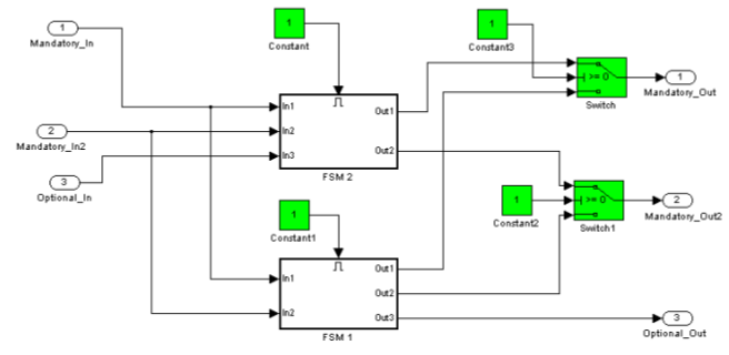
Figure 7 shows the details of the FSM selector subsystem of Figure 6, which has two FSMs, each one executing the behavior of a different variant. Besides the internal variability of each FSM, they also have variability in the configuration of the input and output gates: FSM1 has two inputs and three outputs whereas FSM2 has three inputs and two outputs. Note that both FSMs output their signals to the FSM selector, and, for this reason, we have to use a switch block.
A second approach to model variability in FSM consists of creating a conditional transition to variables that define variabilities. The MATLAB FSMs can have inputs from the dataflow part of a MATLAB/Simulink model. These inputs can be used as conditional variables to perform a transition to one of two states; they can be used as single boolean variables or in expressions involving logic operators. If there are specific states in the machine that implement behavior related to SPL variability, it is possible to create an alternative transition in the FSM so that it can obtain this states depending on the condition associated to the transition. In the cases where the condition is a variable with the value assigned to an FSM input from the dataflow part, the control of the selection variability will require little effort, and it would be possible to be represented as a constant block (the same kind that is being used to enable or disable enabler subsystems in the mechanisms described here).
Figure 8 shows an example of a FSM with variabilities modeled following this approach. In this FSM there are two variants, one that considers only states low_peak and high_peak and other that considers only low_peak and high_peak_counter. If the machine is in the initial state and the variable sine_wave_value is greater than 10, it will change its state. The following state will depend on the boolean variable counter: if this variable is true, the state will be high_peak_counter, or high_peak otherwise.
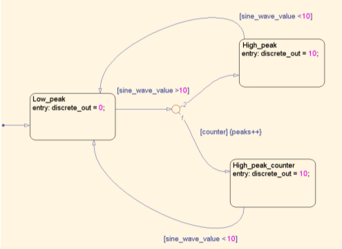
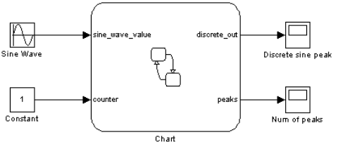
Finally, Figure 8 shows the finite state machine block for the FSM of Figure 9. It is possible to see the inputs of the FSM from the Sine Wave block, the input port that controls the variability (counter) and the machine’s outputs.
4 Modeling Variability of UAV Product Lines Using Simulink
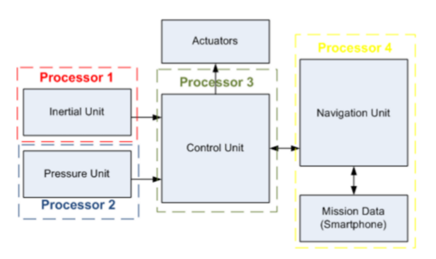
As explained in Section 2.1, Tiriba is an electrically motorized UAV. Modeling its variability as an SPL Simulink model is the main motivation for our investigation. In this section we present some details about the architecture of Tiriba (9) (Figure 10 shows an abstract view of the Tiriba architecture). Note in Figure 10 that Tiriba comprises four processors, which are responsible for the flight control and mission execution. In addition, the source code of each processor is automatically generated from the corresponding Simulink subsystem models:- Pressure subsystem: this subsystem monitors the vertical and horizontal velocities of the vehicle and its altitude.
- Inertial subsystem: this subsystem determines the space position of the vehicle considering its longitude, latitude and altitude.
- Navigation subsystem: this subsystem controls the UAV mission and navigation. Based on the planned flight route the UAV current position, this subsystem computes the actions the vehicle must perform in order to achieve the flight mission.
- Control subsystem: based on the commands sent by the navigation subsystem, this subsystem must computer the suitable parameter values of the actuators, positioning the UAV to the right direction.
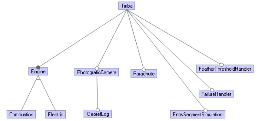
To address the variability space, in this work our domain engineering activity involved a deep study of the UAV domain, interviews with domain specialists, and the restructuring of the Tiriba Simulink model according to the observed variability. The configuration of this variability in the Tiriba Simulink model resulted in a small UAV SPL, represented by the feature model of Figure 11 . In summary, our variability space consists of six optional features (Photographic Camera, GeorefLog, Parachute, EntrySegmentSimulation, FailureHandler, and FeatherThresholdHandler) and one alternative feature Engine that might be further configured as Combustion Based Engine or Electric Engine, but not both of them. Two of the six optional features are related to the UAV payload (Photographic Camera and GeorefLog), one optional feature (Parachute) aims to improve the lifetime of the UAVs, and the remaining three optional features relates to the goals of the missions.
In order to enable an automatic approach for product derivation, we restructured the Tiriba Simulink Model in the points where the optional and alternative features have some influence.
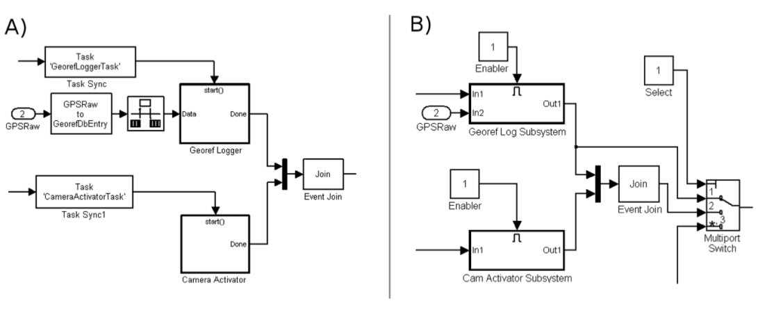
For instance, consider the Photographic camera and Georef log optional features. The UAV camera subsystem won’t be present if the Photographic camera optional feature is not selected for a specific product— and configurations like this are only valid for missions that do no take pictures during the flight. Similarly, the facility of attaching GPS data to the pictures is only available in the cases where the Georef log feature is selected. The changes needed by the Tiriba Simulink model to introduce support for the mentioned variability are as follows. First, the blocks related to both features were removed from the original, single product Simulink model. Then, the corresponding behavior was modeled as enabler subsystems. Finally, we introduced a three-port switch block as a variability mechanism. Using this switch, there are three possible configurations: the selection of both Photographic camera and Georef log, the selection of only Photographic camera, and the absence of both of these features. Figure 12 illustrates how we evolve the original model into the model supporting the SPL variability introduced by the Photographic camera and Georef log features.
Regarding the Parachute feature, the corresponding blocks in the original Simulink model were already specified as an independent subsystem. Therefore, to model the parachute variability, we only had to transform this subsystem into an enabler subsystem, as discussed in Section 2.2. Differently, the variability related to the optional features Entry segment simulation, Feather threshold handler, and Failure handler was specified in the finite-state machine (FSM) that models the Tiriba mission controller unsing the mechanism of transitions conditioned to variables that define variability (as introduced in Section 3). When the feature is Entry segment simulation selected, a simulation is performed whenever the UAV starts a new segment of the mission, in order to find out the better approach to transit between two mission segments. The second feature (Feather threshold handler), when selected, fix the UAV route whenever the vehicle deviates more than a certain limit from the planed mission route. Finally, when the Failure handler feature is selected, the UAV is able to return to specific positions where, for any reason, a picture was not captured during the mission.
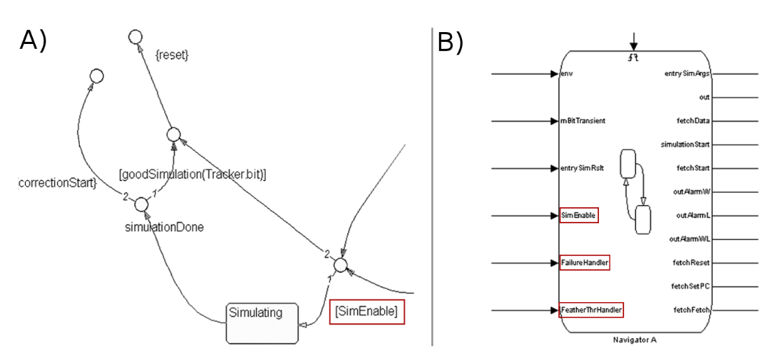
Since the behavior of these features is specified in the mission controller FSM, we introduced alternative flows having boolean variables conditions, which allow us to enable or disable certain flows and states according to the selection or not of the aforementioned features (following the pattern introducted in the section 3 as illustrated by Figures 8 and 9). For instance, the boolean value SimEnable is the conditional that enables (or disable) the behavior related to the Entry segment simulation feature. Therefore, there is a boolean variable for each optional feature related to the mission controller, and the role of these variables is to decide which transitions of the FSM will take place. Figure 13 shows the input values that are assigned to these variables highlighted in red.
There are two valid engine configurations: Combustion based engine and Electric engine. The first leads to a better flight autonomy and higher power when compared to the electric engine, even though introducing complexity to the acceleration controller. This occurs because it is necessary a gradual process for both acceleration and deceleration, target to avoid accidents and the lost of the UAV which eventually occurs due to an engine stop. Another characteristic of combustion based engines is that they are constrained by a low speed limit, and the engine could also stop when the UAV flies at a speed bellow this limit. Electric engines are less restricted, and the acceleration and deceleration might be done abruptly. Moreover, the engine do not stop even when the UAV speed is zero. Therefore, although presenting less autonomy, electric engines are safer, make easier to design and integrate the controller into the UAV, and reduce the maintenance costs. Regarding the Tiriba Simulink model, the engine variability is scattered through two distinct areas: the behavior related to the engine configuration, so that it is possible to configure the maximum and minimal speeds of the UAV; and the behavior related to the acceleration and deceleration of the engine, which is only required by combustion based engines.
4.1 Configuring Tiriba variabilities using Pure::variants
We introduced six variation points to configure the Tiriba Simulink Model so that we could derive instances using Pure::variants. For the Parachute feature, we introduced a boolean parameter and replaced a constant block by a control block, which is connected to the enabler of the parachute subsystem.As mentioned in the previous section, the engine configuration (combustion based or electric based) changes the behavior of two distinct areas (speed and acceleration controllers). For both of them, we introduced a switch as variability mechanism. Then, we configured the control block of these switches with the same variation point, which might assume two distinct values: 0 indicating the selection of the Electric engine feature; and 1 indicating the selection of the Combustion based engine feature.
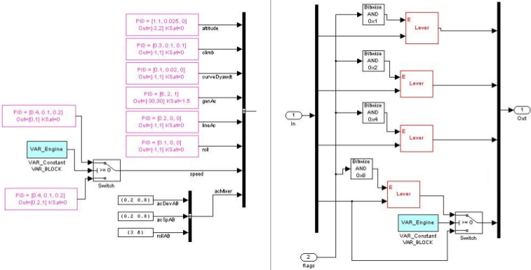
The Figure 14 shows the model in the two areas related to the engine variability. The left side shows the configuration of the minimum speed parameters of each engine: the upper pink block conected to the switch configures the electric engine minimum speed (0) while the lower pink block configures the combustion minimum speed (0.2). The right side shows the aceleration control of each type of engine: the combustion related part (upper port of the switch) needs a Lever subsystem to smooth the desired aceleration level; on the other hand, the electric engine part doesn’t need any block to smooth the desired aceleration; the seted engine aceleration level is the very same as the desired.
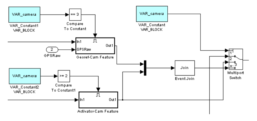
We also configured both Photographic camera and Georef log features using one variation point, whose parameter might assume the values 1 (indicating that none of the features were selected), 2 (indicating that only the Photographic camera feature was selected), and 3 (indicating that both features were selected). We attach this variation point to three control blocks: one attachment to the switch block used as variability mechanism; and two attachments to a comparator block that is connected to the enabler gates of each subsystem that specifies the features Photographic camera and Georef log (see Figure 15.
The remaining variation points, which are related to the UAV mission behavior, might only assume values 0 or 1 (since they address the configuration of optional features). The difference here, when compared to the variation point of the Parachute feature, is that these variation points arise in the finite-state machine (FSM) that specifies the UAV mission. Nevertheless, the conditional gates of Simulink FSMs only accept boolean values as input, while the variation points of Pure::variants are integers. To solve this problem, we implemented a simple integer to boolean converter— when the input value is 0, it returns false; otherwise it returns true.
It was created 6 variation points with the amount of 13 possible values for our Simulink UAV product line. Figure 16 shows the pure::variants feature model and instance model on it’s left side and the variation model with every variation point possible value in its right side.
4.2 Configuring Tiriba variabilities using Hephaestus
It was relatively easy to model Tiriba variability using Hephaestus. The transformations necessary to specify the configuration knowledge were: selectSimulinkBlock and clearVariabilityBlock. In what follows, we detail the configuration knowledge specification.Initially, we related all mandatory blocks to the Tiriba feature, which is the (mandatory) root feature of the Tiriba product line. This triggers the selection of all these mandatory blocks in the final product. We also introduced one feature expression Parachute that selects all Simulink blocks related to this feature.
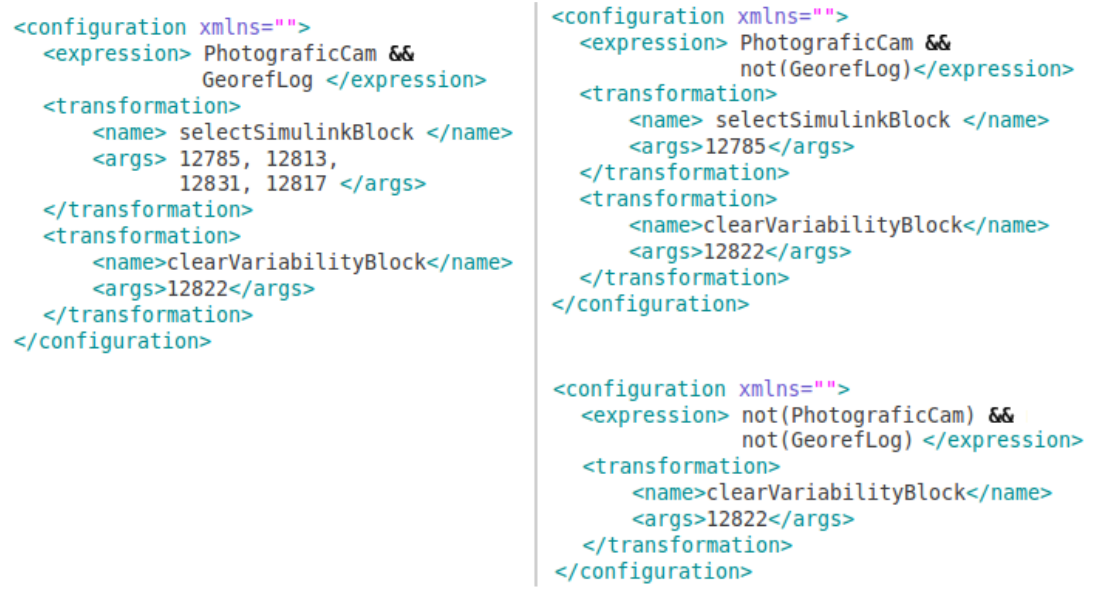
The restruction of the areas related to the Photographic camera and Georef log features were very similar to the restruction shown in Figure 12. Differently of the Parachute feature, the configuration of this features were specified using three feature expressions, since there are three valid combinations of these features and, for each possibility, the variability is solved in a different way. For instance, when both features were enabled, blocks 12785, 12813, 12831, and 12817 must be selected (this blocks are respectively the photografic camera subsystem, georef log subsystem, signal mux and join block) to the final product, and the variability block of id 12822 (a switch block) must be correctly errased from the model. When the Photographic camera is selected and the Georef log feature is not, only blocks 1278 must be selected in the final product, and we must also clear the variability block 12822. Finally, when none of these features are selected, we just must clear the variability block whose identifier is 12822.
The Figure 17 shows the configuration knowledge built for the Photographic camera and Georef log features. In the Figure is possible to see the feature expressions and its implications over the transformations. The only common configuration knowledge part over the three feature expressions is the configuration of the transformation clearVariabilityBlock for the to the variability block switch (id 12822).
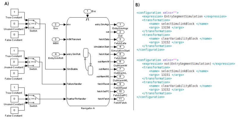
For each mission related feature we created two feature expressions— one for the cases where the feature was selected and another for the cases where the feature was not selected. For instance, if the feature Entry segment simulation is selected, the product derivation selects the 1 value constant block that is connected to the corresponding gate of the FSM. Differently, if the feature Entry segment simulation is not selected, the corresponding 0 value constant block will be selected in the final product. Therefore it was necessary to add two feature expressions for each feature related to de mission, one case the feature is selected and one case it is not. It was also necessary to make use of a switch block as variability mechanism block, which was associated to a clearVariabilityBlock in the configuration knowledge for each feature expression related to the mission. Figure 18 shows on its left side variability mechanisms blocks (as switch blocks) to structure blocks used to assign values of different variability selections; on its right side it is shown the configuration knowledge of the feature Entry segment simulation: there are two expressions (for the case it is selected or not) the selection of one constant block (value 1 if it’s selected or 0 if it’s not) and in both cases the switch variability mechanism block is cleared.
Finally, we specified one feature expression for each valid configuration of the Engine feature. The Tiriba Simulink model parts related to the engine features were restructured to Hephaestus in a very similar way as it was in Pure::variants (see Figure 14). Considering the configuration knowledge, basically it was added three blocks to the be selected (for two different Simulink areas) and two variability blocks to be cleared for the Combustion feature expression. Similarly, in the Electric feature case, one Simulink block is added when Electric feature expression is evaluated as true, and the same two variability blocks must be cleared from the model. Since they are alternative features, Hephaestus guarantees that a valid configuration could not be specified using both features or none of them— and the configuration knowledge do not have to deal with these cases.
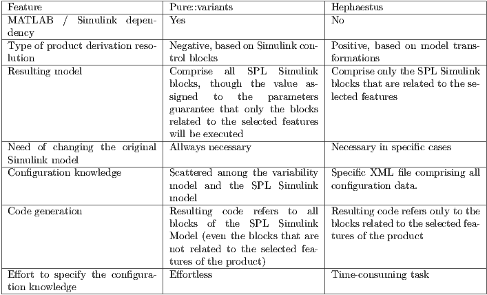
In this section we present a comparison between the implementation of Tiriba variability using Pure::variants and Hephaestus. According to the product derivation process, we realized at leas one significant difference among the compared tools: using Pure::variants the complete set of valid product instances will comprise all blocks (including the blocks introduced to support variability) of the Tiriba product line, regardless of the fact that some features might not be selected. In this case, the product derivation occurs by means of changing the values assigned to the MATLAB workspace parametres of the control blocks. As explained in Section 4, we use contro blocks to enable (or disable) blocks that are related to optional or alternative features, depending on the selection or not of the corresponding feature.
In Hephaestus, the product derivation is built uppon a positive approach, in which the initial Simulink model for the product is empty. Than, after evaluating the proper transformations for a specific instance, new blocks are introduced and modified stepwise. After that, the product derivation connects the selected blocks according to the existing paths (or connections between blocks) of the Simulink product line model. Finally, the product derivation removes all variability mechanisms of the product, in such a way that the resulting model will comprise only the functional variant blocks that are related to the selected features of the SPL instance.
It is important to notice that product derivation using Pure::variants leads to Simulink models that are unnecessarily complex, which in turns produces less efficient generated code— once the Simulink models serve as input for source code generation. Using Hephaestus, the derived instances comprise only the Simulink blocks that are related to the selected features. In this way, there is no dead code motivated by variability management, since the generated code considers only the blocks that are necessary for a specific product. Differently, using Pure::variants the generated code is almost the same for all derived instances, mainly because the Simulink models of the SPL instances allways comprise all blocks. The values assigned to the parameters control the instance’s variabilities, enabling only the execution paths that are valid. Those values are generated from the SPL Simulink control blocks, whose values are specified by Pure::variants.
This is the main advantage of Hephaestus. Since in the embbedded software domain there exist memory constraints, dead code is considered a design fault that should be avoided. So, using Pure::variants, product engineers have to either modify the product specific Simulink model, removing all blocks that are not related to the selected features; or eliminate dead code from the generated source code. In the first case, we could say that the product derivation is only partially automated. Besides that, since both alternatives are difficult to fully automate, they are time consuming and error-prone, particularly in the cases where the resulting Simulink model is complex.
It is reasonably easy to define and evolve the configuration knowledge using both Pure::variants and Hephaestus. Nevertheless, specifying an Hephaestus configuration knowledge requires the extra, time consuming task of finding the identifier of each Simulink block and refering to these identifiers as arguments to the Hephaestus transformations. Moreover, evolving the configuration knowledge in Pure::variants is more intuitive, since all variability is represented in the SPL Simulink model.
Product derivation in both Pure::variants and Hephaestus is effortless. In Pure::variants, after an instance model had been created, a product engineering just have to propagate the configuration using a single command. Similarly, using Hephaestus the product engineering only have to select the product derivation command to derive a product using the selected SPL Simulink model, instance model, and configuration knowledge.
Table 1 summarizes our comparison, presenting the benefits and drawbacks of both tools.
This paper discussed and presented two main results related to the development of software product lines based on Simulink modeling in the domain on UAV. The first and more important was the presentation of a catalog of mechanisms to represent several types of variabilities in Simulink. Then, we used these mechanisms to create, as a proof of concept, a small SPL for part of a real UAV called Tiriba in which we used these mechanisms.
We also studied two tools to support variability and configuration management of SPL modeled using Simulink following a compositional approach and a instrumentation approach supported by, respectively, two tools: Hephaestus and Pure::variants. We discussed the characteristics and the advantages and disadvantages of these two tools. The model of the UAV Tiriba used as the basis for this work is a simplified version, but the proposal can be perfectly applied to the actual software, which could be done by the company that developed Tiriba.
As future work, we intend to apply the knowledge acquired in this work on a real SPL for the family of UAV to which Tiriba belongs. The design of Tiriba is already being modified to develop a product line by Braga et al. (19); In this work, a model of 108 features was created, but it is still not enough for a LPS. This feature model is being extended to later be integrated into a feature model of an LPS based on Tiriba and at least two other UAVs. We are also investigating how an UAV can be certified using a SPL approach (1).
(1)R. T. V. Braga, O. Trindade Jr, K. R. L. J. C. Branco, L. O. Neris, and J. LEE, “Adapting a software product line engineering process for certifying safety critical embedded systems,” in 31st International Conference on Computer Safety, Reliability and Security, 2012, Magdeburg, LNCS 7512, 2012, pp. 352–63.
(2)C. Dziobek, J. Loew, W. Przystas, and J. Weiland, “Functional variants handling in simulink models,” in MathWorks Virtual Automotive Conference, Stuttgart, 2008.
(3)A. Polzer, S. Kowalewski, and G. Botterweck, “Applying software product line techniques in model-based embedded systems engineering,” in Model-Based Methodologies for Pervasive and Embedded Software, 2009. MOMPES’09. ICSE Workshop on. IEEE, 2009, pp. 2–10.
(4)P. Clements and L. Northrop, “Software product lines: Patterns and practice,” Addison Wesley, 2001.
(5)K. Czarnecki and U. Eisenecker, Generative Programming: Methods, Tools, and Applications. Boston, MA: Addison-Wesley, 2000.
(6)K. Kang, S. Cohen, J. Hess, W. Novak, and A. Peterson, “Feature-oriented domain analysis (foda) feasibility study,” Software Engineering Institute, Carnegie Mellon University, Tech. Rep. CMU/SEI-90-TR-021, 1990. [Online]. Available: http://www.sei.cmu.edu/library/abstracts/reports/90tr021.cfm
(7)K. Pohl, G. Böckle, and F. Van Der Linden, Software product line engineering: foundations, principles, and techniques. Springer-Verlag New York Inc, 2005.
(8)E. Pastor, J. Lopez, and P. Royo, “Uav payload and mission control hardware/software architecture,” Aerospace and Electronic Systems Magazine, IEEE, vol. 22, no. 6, pp. 3–8, 2007.
(9)K. Branco, J. Pelizzoni, L. Neris, O. Trindade, F. Osorio, and D. Wolf, “Tiriba— a new approach of uav based on model driven development and multiprocessors,” in Robotics and Automation (ICRA), 2011 IEEE International Conference on. IEEE, 2011, pp. 1–4.
(10)INCT-SEC, “Instituto nacional de sistemas embarcados críticos,” 2008. (Online). Available: http://www.inct-sec.org
(11)J. Dabney and T. Harman, Mastering Simulink. Pearson Prentice Hall, 2004.
(12)G. Botterweck, A. Polzer, and S. Kowalewski, “Using higher-order transformations to derive variability mechanism for embedded systems,” Models in Software Engineering, pp. 68–82, 2010.
(13)J. Weiland, “Configuring variant-rich automotive software architecture models,” in Automotive Electronics, 2006. The 2nd IEE Conference on, march 2006, pp. 73 –80.
(14)A. Leitner, R. Mader, C. Kreiner, C. Steger, and R. Weiß, “A development methodology for variant-rich automotive software architectures,” Elektrotechnik und Informationstechnik, vol. 128, pp. 222–227, 2011.
(15)V. H. Fragal, E. A. O. Junior, and I. M. Gimenes, “Mapping software product line features to unmanned aerial vehicle models,” in 1st Brazilian Conference on Critical Embedded Systems, 2011.
(16)C. Kästner, S. Apel, and M. Kuhlemann, “Granularity in software product lines,” in Proceedings of the 30th international conference on Software engineering, ser. ICSE ’08. New York, NY, USA: ACM, 2008, pp. 311–320. (Online). Available: http://doi.acm.org/10.1145/1368088.1368131
(17)M. Torres, U. Kulesza, M. Sousa, T. Batista, L. Teixeira, P. Borba, E. Cirilo, C. Lucena, R. Braga, and P. Masiero, “Assessment of product derivation tools in the evolution of software product lines: an empirical study,” in Proceedings of the 2nd International Workshop on Feature-Oriented Software Development, ser. FOSD ’10. New York, NY, USA: ACM, 2010, pp. 10–17. (Online). Available: http://doi.acm.org/10.1145/1868688.1868691
(18)R. Bonifácio, L. Teixeira, and P. Borba, “Hephaestus: A tool for managing product line variabilities,” in Third Brazilian Simposium on Components, Architecture, and Software Reuse, 2009, pp. 26–34.
(19)R. T. V. Braga, O. Branco, K. R. L. J. C. Trindade Jr, P. C. Masiero, L. O. Neris, and M. Becher, “The prolices approach to develop product lines for safety-critical embedded systems and its application to the unmanned aerial vehicles domain,” CLEI Electronic Journal, vol. 15, pp. 1–13, 2012.

