An efficient version of the RMA-11 model

Ezzatti, Pablo; Fossati, Mónica; Piedra-Cueva, Ismael

Services on Demand

Journal

Article

Automatic translation

CLEI Electronic Journal

On-line version ISSN 0717-5000

CLEIej vol.14 no.2 Montevideo Aug. 2011

An efficient version of the RMA-11 model

Pablo Ezzatti
Facultad de Ingeniería, Universidad de la República,
Montevideo, Uruguay, 11300,
pezzatti@fing.edu.uy
Mónica Fossati
Facultad de Ingeniería, Universidad de la República,
Montevideo, Uruguay, 11300,
mfossati@fing.edu.uy
Ismael Piedra-Cueva
Facultad de Ingeniería, Universidad de la República,
Montevideo, Uruguay, 11300,
ismaelp@fing.edu.uy

Abstract

RMA-11 is a numerical model widely used for studing the transport of constituents and water quality in rivers and estuaries. When applied to large water systems like the Río de la Plata, RMA-11 demands long execution times to compute a simulation. This paper presents the analysis of the computational efficiency for the RMA-11 applied to a transport model of the Río de la Plata, and introduces a proposal for improving the efficiency by using high performance computing techniques. The improved implementation modifies the linear system resolution methodology implemented in the model. A high performance computing strategy was applied to the FRONTALL routine of the RMA-11, by changing their logical structure and using a sparse storage format. The experimental results obtained when solving representative test cases show a significant improvement on the performance, achieving significant gains in computational speed: the execution time of the implemented version decreased up to one third of the time of the original implementation.

Keywords: computational fluid dynamics, transport numerical model, high performance computing

Abstract

El RMA-11 es un modelo numérico ampliamente utilizado para estudios del transporte de constituyentes y de la calidad del agua en ríos y estuarios.
Cuando se aplica este modelo a cuerpos de agua de grandes dimensiones, como es el caso del Río de la Plata, el RMA-11 insume tiempos de ejecución largos para computar las simulaciones.
Este artículo presenta un análisis de la eficiencia del modelo RMA-11 aplicado al modelado del transporte de sustancias del Río de la Plata, además se presenta una propuesta para mejorar el desempeño del modelo utilizando técnicas de computación de alto desempeño.
La implementación propuesta modifica la estrategia para resolver los sistemas lineales provista en el modelo original.
En particular, estrategias de computación de alto desempeño son aplicadas a la rutina FRONTALL del RMA-11, cambiando su estructura lógica y empleando formatos de almacenamiento disperso. Los resultados experimentales obtenidos al resolver casos de prueba representativos muestran mejoras significativas en el desempeño, alcanzando ganancias importantes en los tiempos de ejecución: el tiempo de ejecución de la versión propuesta es un tercio del tiempo de la versión original.

Spanish Keywords: Computación de dinámica de fluidos, modelo numérico de transporte, computación de alto desempeño.

Received 2011-May-30, Revised 2011-Aug-30, Accepted 2011-Aug-30

1 Introduction

The research applying numerical models to solve environmental fluid dynamics problems has increased notably over the last decades. In Uruguay, numerical models have been used to study the hydrodynamic of the Río de la Plata and its Maritime Front since the 1990s decade. These studies were carried out applying and developing several numerical models in the Instituto de Mecánica de Fluidos e Ingeniería Ambiental (IMFIA) of the Facultad de Ingeniería. The initial models based on finite differences schemes [1] were later replaced by more accurate models using the finite element methods (FEM) methodology.

Currently, the RMA finite element method set is used to model the Río de la Plata. This family of methods includes the two-dimensional vertically integrated hydrodynamic model RMA-2, the three dimensional baroclinic hydrodynamic model RMA-10, and the water quality model RMA-11 [2]. All these models have shown accurate modeling capabilities to represent the dynamic flow and water quality in the Río de la Plata, obtaining correct representations of the physics processes in the model and the coastline representation, while being able to work with irregular grids and different types of elements. However, an important drawback of the FEM approach is the lose of computational efficiency. This drawback limits the application of RMA model to large dimension realistic scenarios and it also makes it hard to implement a three-dimensional hydrodynamic version of RMA or to use with high resolution meshes.

High performance computing (HPC) techniques are based on maximizing the available computer capabilities as well as minimizing computing requirements to solve a particular problem. In order to achieve these objectives, specific methods are developed to reduce the resources requirements taking into account the computer architecture (e.g. memory, processors, connections).

In this work, HPC techniques are applied to the RMA-11 model in order to develop an efficient version that allows reducing the computing time required to perform the simulation of large scenarios.

The methodology for improving the RMA-11 model performance involves the following steps. First, a study of the execution time of the original routines was undertaken to indentify the possibles bottlenecks. After that, several improvement were devised and implemented. Finally, the improved version was evaluated by comparing the computational performance and the numerical results with those obtained with the original version for several test cases that model the Río de la Plata.

The paper is organized as follows. The RMA-11 model is described in Section 2. In Section 3, the analysis of the execution time for the original version of the model is presented. The new improved version of RMA-11 is introduced in Section 4, just before presenting the computational and numerical evaluation in Section 5. Finally, in Section 6 the conclusions and some lines of future work are presented.

2 The numerical model

RMA-11 is a widely used numerical model for engineering applications. It is a finite element water quality model for simulation of one-, two-, and three-dimensional estuaries, bays, lakes and rivers, which has been applied to the Río de la Plata [3] as well as other water systems around the world [4, 5]. RMA-11 was designed to accept velocities and bathymetry input files from the outputs of the two-dimensional hydrodynamic model (RMA-2) and the three-dimensional stratified flow model (RMA-10). The provided hydrodynamic data is used to solve the advection-diffusion-reaction constituent transport Equation (1), which calculates the spatial and temporal distribution of water constituent concentration $c$ using a space time coordinates system $(x,t)$ and a matrix $D$ with the diffusion coeficients.

-δ δtc(x,t) +u ∇c(x,t) - ∇ (D(x,t)∇c (x,t)) = f(c(x,t))

(1)

The second term of Equation (1) represents the advection process and the third term represents the diffusion process of the water constituent studied. The two and three-dimensional advection diffusion equations are simulated for conservative and decaying constituents. The decay or growth function depends on the concentration, and they are included in the reaction term. The term on the right, $f(c(x,t))$ , represents the source and the reaction component of the equation, used to left open the possibility of including nonlinear dynamics.

The RMA-11 model is able to represent irregular boundary configurations, variable element sizes, and the wetting and drying of shallow portions of the modeled region. The model may be executed in a steady state or in a dynamic mode. The velocity fields used to solve the advection diffusion equations may be constant or interpolated from an hydrodynamic output file. The model operates independently of the timesteps in the hydrodynamic model, and if it is necesary, the input data is automatically interpolated. The source pollutant loads may be an input of the system either at discrete points, over the elements, or as fixed boundary values.

The RMA-11 model is able to compute more than 15 constituents simultaneously. The load, the initial conditions and the decay conditions must be defined for each constituent. The model can simulate the temperature with a full atmospheric heat budget at the water surface, the nitrogen and phosphorous cycles, the biological oxygen demand and dissolved oxygen relationship, the algae growth and decay, the cohesive suspended sediment or non-cohesive suspended sediment such as sand, and other non-conservative constituents. Another important feature of the RMA-11 model is the fully implicit resolution scheme implemented to solve time-dependant problems. This feature allows using long time steps even in a dynamic scenario with a high resolution grid.

The model implementation consists of several modules. Most of the routines are written in the FORTRAN 77 language, while recently added modules are implemented in FORTRAN 90. The model is available for several operative systems, such as Linux, Unix and Windows (NT, XP and Server).

Algorithm 1 presents a pseudocode of the original RMA-11 implementation.

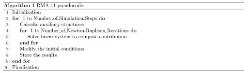
The first step of the Algorithm 1 corresponds to the initialization stage, where RMA-11 reads the grid and global parameters from the input files. After that, the main loop of the program is executed (steps 2 to 9 in Algorithm 1). In each iteration, the computations needed to simulate a time step are performed. The time step process includes the resolution of the finite element non-linear system of equations using as the initial condition the results obtained in the previous step. The Newton-Raphson (NR) method is used to solve the non-linear system of equations (steps 4 to 6), which implies the resolution of a linear system of equations on every iteration of NR. The RMA-11 model allows defining the convergence criterion and the maximum number of iterations for the method. In every dynamic application the FEM requires computing the nodal values of the mesh elements at each time step (or at each Newton-Raphson iteration for a non linear problem). These values are assembled and later used for generating the stiffness matrix. In the RMA-11 model, these tasks are performed in the step 5 of Algorithm 1 by the FRONTALL routine and several subroutines implemented in order to efficiently determine the value of coefficients. The selection is done at runtime and the selected subroutine depends on the element type and form that is being processed. A Gauss quadrature method is used to solve the integrals needed to compute the nodal values. Later, the initial conditions of the next iteration step are modified (step 7) and the results are stored (step 8). Finally, the finalization stage (step 10) performs several tasks: it stores the final results, releases the computational resources and closes the open files.

The linear system resolution strategy defined in the RMA-11 model is the frontal method introduced by B. Irons [6], which was later extended to non-symmetric matrices by P. Hood [7]. The frontal methods are versions of the Gaussian elimination, directly related with the FEM strategy, and designed to attenuate memory requirements of the standard strategies. The methodology of the frontal method consists in loading the matrix into pieces (called fronts) in the system memory. This feature was proposed to allow the resolution of large linear systems implemented in the numerical methods with the hardware available in the 1970s. When simulating several constituents, the linear system has several unknown vectors and the method can resolved simultaneously. This situation does not affect the factorization stage, but when simulating several constituents the method needs to perform as many substitutions as the number of linear systems that have to be solved.

The high accurate results obtained with the RMA-11 are overshadowed by the high computional cost needed to simulate the transport of sustances over large scenarios. In this context, the use of HPC techniques is suggested to improve the computational efficiency. However, a survey conducted on this line of research allows to conclude that there have not been published any papers about the application of HPC techniques to the RMA-11 model. Thus, there is still room to contribute in this line of research, by proposing a highly efficient RMA-11 implementation that allows tackling problem instances with increasing size.

3 Computational cost

This section presents the results obtained in the evaluation of the original version of the RMA-11.

3.1 Test cases for the transport of substances in the Río de la Plata

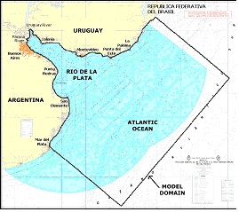
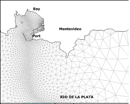
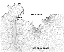
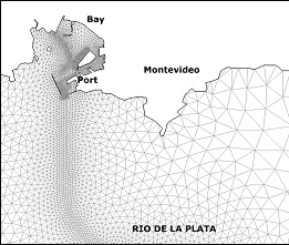
Several test cases were defined to evaluate both the original and the new routines implemented in the RMA-11. Six scenarios with different numbers of elements, nodes and simulated constituents were used, considering three different grids of the Río de la Plata domain (called M1, M2 and M3). The main difference among the grids is their resolution in coastal zone of Montevideo. Figure 1 (a) shows the model domain and the details of the M1, M2, and M3 grids near Montevideo are presented in Figures 1 (b), 1 (c), and 1(d), respectively.

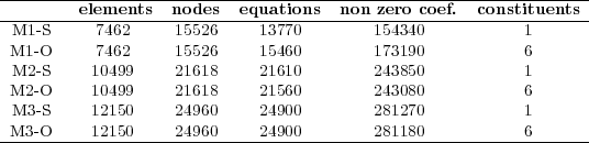
Figure 1: (a) Location of the studied area and model domain. (b) M1 (c) M2 and (d) M3, grid details in the coastal zone of Monteideo.

In addition to this, two RMA-11 simulation types were defined for each grid. In the executions with type S, the model computes only one constituent, the cohesive suspended sediment transport. In the executions with type O, the model computes six constituents: the dissolved oxygen, the bio-chemical oxygen demand, the organic nitrogen, the ammonium, the nitrate and the nitrite. The hydrodynamic model was validated with all these grids using empirical results, water levels and velocities measured in different areas of the Río de la Plata [8, 9]. The main characteristics of the test cases used in this work are presented in Table 1, showing for each grid the number of elements, grid nodes, equations, non zero coefficients of the matrix and simulated constituents.

Table 1: Main characteristics of the test cases for the transport of substances in the Río de la Plata.

-------------------------------------------------------------------- ---------elements---nodes---equations--non--zero coef.-constituents-- M1 -S 7462 15526 13770 154340 1 M1 -O 7462 15526 15460 173190 6 M2 -S 10499 21618 21610 243850 1 M2 -O 10499 21618 21560 243080 6 M3 -S 12150 24960 24900 281270 1 -M3--O-----12150-----24960----24900--------281180-----------6--------

3.2 Development and execution platform

All tests were performed on a Dell multicore computer with two processors Pentium IV at 2.8 GHz, 1 GB of RAM, and using the Debian 4.1.1 Linux operating system. The Intel Fortran 9.0 compiler was used.

3.3 Runtimes of the RMA-11 stages

To perform the runtime study, the RMA-11 model is divided according to the five different stages specified in Algorithm 1: initialization, calculation of auxiliary structures, resolution of the linear systems, modication of the initial conditions, and finalization.

In this analysis, the M3-O test case is used since it represents the longest scenario, using a maximum of 4 iteration steps for the stop criterion in the Newton-Raphson method. The computation involves 12,150 elements and 24,960 nodes, and it computes 6 constituents.

Table 2 summarizes the average execution times and the standard deviation ( $σ$ ), obtained in 10 independent executions for each of the RMA-11 model stages.

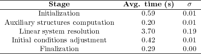
Table 2: Execution times of the RMA-11 stages.

---------------------------------------------------- ------------Stage--------------Avg.--time--(s)----σ--- Initialization 0.59 0.01 Auxiliary structures computation 0.20 0.01 Linear system resolution 3.70 0.19 Initial conditions adjustment 0.42 0.01 ----------Finalization----------------0.29-------0.00--

The analysis of the runtimes in Table 2 shows that the stiffness matrix computation and resolution (linear system resolution) is the most demanding stage. Moreover, the execution times of the initialization and finalization stages are independent of the number of simulation steps. So, it is expected that in larger simulations the influence of these execution times will be smaller than in the evaluated case. In fact, in the test case presented, the execution time of the initialization and finalization stages are not significant (they are shorter than those required to perform one iteration step of the Newton-Raphson method). A similar situation happens for the stage that computes the auxiliary structures and the stage that adjust the initial conditions, which are executed only once for each time step. However, the stiffness matrix computation is performed by the FRONTALL routine in every Newton-Raphson execution to solve the nonlinear system of equations. FRONTALL is the routine that demands the higher computing cost. Thus, a second analysis was performed to evaluate the execution time of the steps inside the FRONTALL routine.

3.4 Execution time of the FRONTALL routine

The FRONTALL routine uses the frontal method to solve the linear system, so it does not need to compute all the coefficients of the stiffness matrix to start the factorization. In order to use less memory, the method evaluates several elements, computing the coefficients and factoring the different fronts in the stiffness matrix. The execution time of the three logical stages of the FRONTALL routine was analyzed and computed, in order to identify the critical sections of the code. The logical stages involved are the coefficient computation, the factorization of the different fronts in the sparse matrix, and the substitutions. The execution time of each stage was calculated adding the execution time of its components. For example, the execution time of the factorization stage was computed as the sum of the execution times needed to factorize each front.

Table 3 presents the average execution times and standard deviation ( $σ$ ), obtained in 10 independent executions, for each stage of the FRONTALL routine.

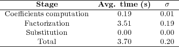
Table 3: Execution time of the stages of the FRONTALL routine on the M3-O test case.

-------------------------------------------- ---------Stage----------Avg.-time-(s)---σ--- Coefficients computation 0.19 0.01 Factorization 3.51 0.19 Substitution 0.00 0.00 ---------Total---------------3.70-------0.20-

The results on Table 3 allow to conclude that the factorization is the stage which demands the longest execution time in the FRONTALL routine.

As a conclusion of this section, the application of HPC techniques should focus on the FRONTALL routine, specially in the factorization stage.

4 High performance computing in RMA-11

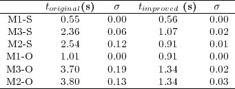
This section describes the application of high performance computing techniques on the FRONTALL routine of the RMA-11 model. The logical structure of the FRONTALL routine was modified in order to design a new efficient version. First, the values of all coeficients are calculated. Then, a sparse storage strategy is applied to the stiffness matrix to reduce the space needed for large problem instances. Finally, a specialized method is used to factorize and solve the linear systems.

4.1 Stages of new FRONTALL routine

The new implementation of the FRONTALL routine is logically split into three independent stages: the coefficient calculation, the matrix generation, and the system resolution:

Coefficient calculation: the coefficients for each element are computed and stored in an auxiliary structure.
Matrix generation: the coefficients are filtered and reordered to generate a sparse matrix in some format.
System resolution: the factorization and resolution of the linear system are performed.

These three stages are commented in detail in the following subsections.

4.2 Coefficients calculation

The coefficient calculation step performs one iteration over the grid elements to compute the local stiffness matrix. This stage uses the original RMA-11 routines to calculate the coefficients and to store them in a local structure. Then, the computed values are stored in a new auxiliary global structure: an open hash table.

The hash strategy is based on separating the dataset in a specific amount of classes, called buckets. Thus, a dispersion function that returns only one bucket class for each dataset object is required. When open hashes are used, each bucket uses a list of elements. To improve the storing strategy, the dispersion function is defined by the row of the store coefficient (see Equation 2). The list of buckets is composed of several nodes, which are duplets formed by an indicator column and a coefficient value.

f (coef ) = i dispersion ij

(2)

The dispersion function is applied to each coefficient ( $coefij$ ) for loading the data. Once the hash bucket is obtained (the value of $i$ ) their list is checked in order to search the value with the same column indicator (the value of $j$ ). If this value exists, the calculated coefficient is added to the previous one. Otherwise, a new node containing the value of the calculated coefficient and the corresponding column indicator is added at the end of the list.

At the end of this stage all the coefficients are available in a simple sparse format matrix. However, coefficients equal to zero could exist due to the matrix construction methodology.

4.3 Matrix generation

In the second stage, several depuration tasks are performed. This process is needed in order to apply the resolution method that is used. The depuration tasks implemented include filtering the zero coefficients, ordering the coefficients, and changing the sparse storage strategy to recover the matrix in the format required by the next stage.

Although the design of this stage is generic to any solver of linear systems, a particular version was implemented in the new version of the routine to satisfy the requirements of the employed solver. In this case, the zero coefficients are filtered but no order is established to the coefficients, because the simple sparse storage format is sufficient for the requirements of the next stage.

4.4 System resolution

The last stage of the new routine performs the factorization of the linear system of equations and its resolution. The version 4.6.3 of the MUMPS library [10, 11] is used to factorize and to solve the system. MUMPS implements a multifrontal method using the BLAS library. This method outperforms the frontal method on the use of different memory levels [12], specially allowing to exploit the cache memory. In the new routine for solving the linear system, the BLAS implementation by K. Goto [13] was used.

5 Performance evaluation

This section presents the results obtained in the evaluation of the improved version of the RMA-11 model. The analysis was performed on the computational platform presented in Section 3.2 for solving the test cases described in Section 3.1. First, the evaluation of the numerical results obtained with the improved version for solving the M3-O case using a simulation with 544 time steps is analyzed. Then, a comparison between the execution times obtained with the RMA-11 original version and the improved version for all test cases is presented.

5.1 Numerical results

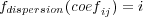
For the Río de la Plata test scenarios, the coefficient matrices are highly ill-conditioned. Small perturbations in the calculation may therefore deviate the numerical results in a few simulation steps. In order to validate the proposed routine, the numerical results obtained with it are compared with the results obtained with the original routine for the M3-O case simulation. The corresponding simulation time steps were 30 minutes and since 544 steps were simulated, 136 hours of execution time were required. Since the errors are acumulative, the comparison is performed on the results of the last step.

Table 4 presents for each simulated constitutent the distance measured with the 2-norm (diff) and the maximum difference (max diff), between the results of the last simulation time step for both model versions. The results show that the differences on the final numerical values are below $1.00 × 10-3$ , meaning that both RMA-11 model versions computed, in practice, the same results. Therefore, the analysis allows to conclude that the modifications implemented in the RMA-11 model did not affect the quality of results obtained with the numerical model.

Table 4: Differences on the numerical results between the original and the proposed versions.

----------------------------------------- -constituents---diff-(2--norm-4)---max--diff-5-- OD 4.53× 10-4 5.15× 10-5 BOD 1.10× 10-5 3.05× 10-6 N org 7.19× 10-6 2.86× 10-6 NH3 7.50× 10-7 1.91× 10-8 NO2 2.30× 10-7 8.94× 10-8 -----NO3--------3.15×-10-----4.47×-10----

5.2 Execution time evaluation

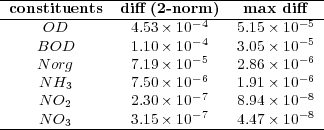
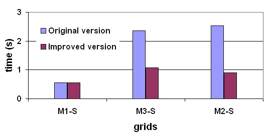
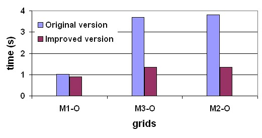
The evaluation of the execution time of the model was performed in two types of experiments. First, a comparison between the execution time of the original and the improved FRONTALL routine was performed. Second, the execution time of the whole model in its original and improved versions were compared.

Table 5 compares the execution time of the original and the improved FRONTALL routine for the six test cases considered in the analysis, reporting the average execution time for each routine version and the standard deviation computed in 10 independent executions. The results are presented grouped by number of simulated constituents and in growing order of computational cost of the original version.

Table 5: Execution time of the original and the improved FRONTALL routine for the six test cases studied.

------------------------------------------- --------toriginal(s)---σ----timproved-(s)---σ--- M1 -S 0.55 0.00 0.56 0.00 M3 -S 2.36 0.06 1.07 0.02 M2 -S 2.54 0.12 0.91 0.01 M1 -O 1.01 0.00 0.91 0.00 M3 -O 3.70 0.19 1.34 0.02 -M2--O------3.80-----0.13------1.34------0.03--

The execution time with the improved FRONTALL routine using the M3-O test case are presented in Table 6, presenting the total execution time as well the time requiered to perform each of the three stages of the routine.

Table 6: Execution time of the stages of the improved FRONTALL routine on M3-O test case.

------------------------------------- -------Stage----------Time-(s)----σ-- Coefficient calculation 0.66 0.02 Re- order 0.00 0.00 Resolution 0.68 0.02 --------Total-----------1.34-----0.02-

The analysis of the results demonstrate that the original FRONTALL routine takes almost 3 times longer than the improved routine. In addition to this, the comparison of the execution times of the factorization stage of the original routine with the sum of the times requiered to load in the auxiliary structure, reorder, factorization and linear system resolution of the improved FRONTALL routine shows that the speedup in the execution times has a factor of $4x$ .

In order to evaluate the impact of the improved FRONTALL routine in the RMA-11 model, a simulation with, the original and the improved versions was performed, evaluating the runtime required to perform a 544 time steps simulation of the M3-O test case. The original version needed 124.7 minutes, while the improved version took 56.1 minutes to perform the simulation. The results clearly show that the execution time of the improved version is less than half the time required by the original version.

5.3 Scalability of the improved FRONTALL version

Figure 2 presents a study of the speedup and the scalability of the improved version of FRONTALL routine with different grids.

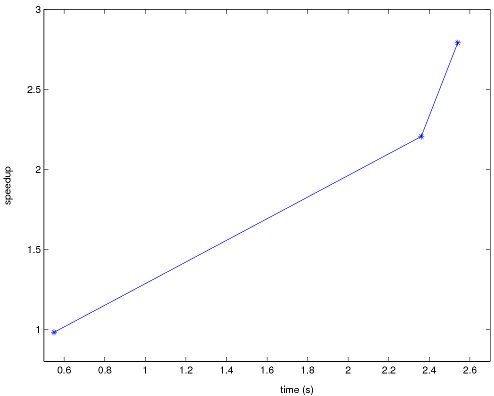
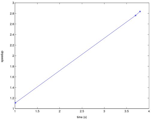
Figure 2: (a) Runtime of the FRONTALL routine for S grids. (b) Speedup of the improved version for S grids (c) Runtime of the FRONTALL routine for O grids. (d) Speedup of the improved version for O grids.

The graphics in Figure 2 show that the improved version has a good scalability behavior, since the improved version obtains the higher values of speedup when the original version needs larger execution time. In addition, the results for the O cases, which are most dificult to simulate, presents large improvement values.

There is another positive feature (not formalized) of the new version of the RMA-11 model. The amount of RAM memory required for the same simulation is smaller in the new version than in the original one, due to the sparse storage approach used.

6 Concluding remarks and future work

This work has evaluated the RMA-11 numerical model to simulate the substance transport in the Río de la Plata. The main contribution is an improved version of the model, based on an alternative strategy for solving the linear systems of the model.

The methodology used in the improved RMA-11 implementation consists in separating the generation of the stiffness matrix from the system resolution stage. An auxiliary hash structure is incorporated to temporarily store the coefficients. After that, a new stage performs the reordering and the consolidation of the coefficients in a sparse storage format. Finally, the linear systems of equations is solved using the MUMPS 4.6.3 library with the optimized BLAS library implemented by K. Goto.

The numerical results obtained with the original and the new improved routine for solving medium size simulations were compared. The differences between the numerical values were always less than $1.00× 10-3$ , showing that the improved methodology for solving the linear systems is able to compute similar results to the original version.

Regarding the computational performance, the execution time evaluation showed that the improved version of the FRONTALL routine is clearly more efficient than the original version. The performed tests demonstrated that the original version required three times the runtime of the new version to perform the same simulation.

In order to model the Río de la Plata substance transport, long periods of time (almost one year) must be simulated. Thus, the improved version of the RMA-11 model reduces considerably the time required to carry out this type of studies. The performance improvement achieved with the new RMA-11 version allows the researchers to expand its applicability to large scenarios, improving the resolution of the grids and executing large simulations in reasonable execution times.

Several aspects about the computational performance improvement of RMA-11 model could be explored in more detail. A first issue not covered in this study is the formalization of the memory requirements of the original and the improved version. Since the stiffness matrix generation process can be significantly improved, the reutilization of the information from previous steps to improve the matrix coefficients calculation should be study.

Other relevant topics that should be considered are the evaluation of the ordering techniques such as minimum degree [14] and nested dissection [15], hybrid [16], and the use of other libraries to solve sparse linear system such as the Watson Sparse Matrix Package presented by A. Gupta [17].

Finally, the application of parallel computing techniques shall be analyzed. There are many options to apply parallelism in the matrix generation process, in the linear systems solves, and also by including domain decomposition strategies to the whole RMA-11 model.

References

[1] R. Guarga, E. Kaplan, S. Vinzón, H. Rodríguez, and I. Piedra-Cueva, “Aplicación de un modelo de corrientes en diferencias finitas al Río de la Plata,” Revista Latinoamericana de Hidráulica. San Pablo, Brasil, 1992.

[2] I. King, “Rma-11: A three-dimensional finite element model for water quality in estuaries and streams version 2.5,” Dept. of Civil and Environmental Engineering, University of California Davis, California, Tech. Rep., 1997.

[3] I. Piedra-Cueva, E. Lorenzo, and M. Fossati, “Modelación numérica del futuro emisario punta lobos (Montevideo),” in XX Congreso Latinoamericano de Hidráulica, La Habana, Cuba, 2002.

[4] M. Weinberg, C. Lawrence, J. Anderson, and J. Randall, “Biological and economic implications of sacramento watershed management options,” in Journal of the American Water Resources Association, vol. 38, 2002, pp. 367–384.

[5] L. Liu, M. Phanikuma, S. Molloy, R. Whitman, D. Chively, M. Nevers, D. Schwab, and J. Rose, “Modeling the transport and inactivation of e. coli and enterococci in the near-shore region of lake michigan,” Environmental Science & Technology, vol. 40, pp. 5022–5028, 2006.

[6] B. M. Irons, “A frontal solution program for finite element analysis,” International Journal for Numerical Methods in Engineering, vol. 2, pp. 5–32, 1970.

[7] P. Hood, “Frontal solution program for unsymmetric matrices,” International Journal for Numerical Methods in Engineering, vol. 10, pp. 379–400, 1976.

[8] I. Piedra-Cueva and M. Fossati, “Residual currents and corridor of flow in the Río de la Plata,” Applied Mathematical Modelling, vol. 31, pp. 564–577, 2007.

[9] M. Fossati and I. Piedra-Cueva, “Numerical modelling of residual flow and salinity in the Río de la Plata,” Applied Mathematical Modelling, vol. 32, pp. 1066–1086, 2008.

[10] P. Amestoy, “Recent progress in parallel multifrontal solvers for unsymmetric sparse matrices,” in Proceedings of the 15th World Congress on Scientific Computation, Modelling and Applied Mathematics, IMACS 97, 1997.

[11] P. Amestoy, I. Duff, , J. Koster, and J.-Y. L’Excellent, “A fully asynchronous multifrontal solver using distributed dynamic scheduling,” SIAM Journal of Matrix Analysis and Applications, vol. 23, pp. 15–41, 2001.

[12] A. Guermouche, J.-Y. L’Excellent, and G. Utard, “Impact of reordering on the memory of a multifrontal solver,” Parallel Comput., vol. 29, pp. 1191–1218, September 2003.

[13] K. Goto, 2009, high-Performance BLAS,http://www.cs.utexas.edu/users/kgoto/. Available at May 2011.

[14] J. Liu, “Modification of the minimum-degree algorithm by multiple elimination,” ACM Transactions on Mathematical Software, vol. 11, no. 2, pp. 141–153, 1985.

[15] E. Rothberg and S. C. Eisenstat, “Node selection strategies for bottom-up sparse matrix ordering,” SIAM Journal of Matrix Analysis and Applications, vol. 19, no. 3, pp. 682–695, 1998.

[16] G. Karypis and V. Kumar, “A coarse-grain parallel formulation of multilevel k-way graph partitioning algorithm,” in Parallel Processing for Scientific Computing. SIAM, 1997.

[17] A. Gupta, “Recent advances in direct methods for solving unsymmetric sparse systems of linear equations,” ACM Transactions on Mathematical Software, vol. 28, no. 3, pp. 301–324, 2002.