


Servicios Personalizados
Revista

Articulo
 Inglés (pdf)
 Articulo en XML
 Referencias del artículo
 Curriculum ScienTI
Links relacionados
Compartir

 Permalink
CLEI Electronic Journal
versión On-line ISSN 0717-5000
CLEIej vol.14 no.1 Montevideo abr. 2011
Abstract
Traditional classification algorithms consider learning problems that contain only one label, i.e., each example is associated with one single nominal target variable characterizing its property. However, the number of practical applications involving data with multiple target variables has increased. To learn from this sort of data, multi-label classification algorithms should be used. The task of learning from multi-label data can be addressed by methods that transform the multi-label classification problem into several single-label classification problems. In this work, two well known methods based on this approach are used, as well as a third method we propose to overcome some deficiencies of one of them, in a case study using textual data related to medical findings, which were structured using the bag-of-words approach. The experimental study using these three methods shows an improvement on the results obtained by our proposed multi-label classification method.
Portuguese abstract
Algoritmos de classificação usualmente consideram problemas de aprendizado que contêm apenas um único rótulo, i.e., cada exemplo é associado a um único valor para o atributo meta. No entanto, um número crescente de aplicações envolve dados para os quais múltiplos atributos metas estão associados. Para esses casos, são utilizados algoritmos de classificação chamados multirrótulo. A tarefa de aprendizado com esses dados pode ser resolvida por métodos que transformam o problema em diversos problemas de classificação monorrótulo. Neste trabalho, dois métodos tradicionais baseados nessa abordagem são utilizados, bem como um terceiro método por nós proposto para superar algumas deficiências desses métodos. Também é realizado um estudo de caso utilizando dados textuais relacionados a laudos médicos, os quais foram estruturados utilizando a abordagem bag-of-words. O estudo experimental utilizando esses três métodos mostra uma melhora na qualidade de predição obtida pela utilização do método de classificação multirrótulo proposto neste trabalho.
Keywords: machine learning, multi-label classification, binary relevance, label dependency.
Portuguese Keywords: aprendizado de máquina, classificação multirrótulo, binary relevance, dependência de rótulos.
1 Introduction
Traditional single-label classification methods are concerned with learning from a set of examples that are associated with a single label  from a set of disjoint labels
  ,
,  [9, 1]. However, there are several scenarios where each instance is labeled with more than one label at a time, i.e., each instance
  is associated with a subset of labels
  . In this case, the classification task is called multi-label classification.
Multi-label classification has received increased attention in recent years, and has been used in several applications such as music categorization into emotions [8, 11], semantic images and video annotation [2, 18], bioinformatics [5, 15] and text mining [14], to mention just a few.
Existing methods for multi-label classification fall into two main categories, which are related to the way that single-label classification algorithms are used [13]:
- problem transformation; and
- algorithm adaptation.
Problem transformation methods map the multi-label learning task into one or more single-label learning tasks. When the problem is mapped into more than one single-label problem, the multi-label problem is decomposed into several independent binary classification problems, one for each label which participates in the multi-label problem. This method is called Binary Relevance (BR). The final multi-label prediction for a new instance is determined by aggregating the classification results from all independent binary classifiers. Moreover, the multi-label problem can be transformed into one multi-class single-label learning problem, using as target values for the class attribute all unique existing subsets of multi-labels present in the training instances (the distinct subsets of labels). This method is called Label Power Set (LP). Any single-label learning algorithm can be used to generate the classifiers used by the problem transformation methods. Algorithm adaptation, on the other hand, extends specific learning algorithms in order to handle multi-label data directly.
The community has been working on the design of multi-label methods capable of handling the different relationships between labels, especially label dependency, co-occurrence and correlation. Some of these label relationships can be extracted from the training instances. In the LP method, for example, inter-relationships among labels are mapped directly from the data, since all the existing combinations of single-labels present in the training instances are used as a possible label in the correspondent multi-class single-label classification problem. In this context, the Binary Relevance method has been strongly criticized due to its incapacity of handling label dependency information [10]. In fact, the BR method assumes that each single label is independent of the others, which makes it simple to implement and relatively efficient, although incapable of handling any kind of label relationship. Nevertheless, the Binary Relevance framework has several important aspects that help the development of new methods, which can be used to incorporate label dependency aiming to accurately predict label combination while keeping the simplicity and efficiency of the BR framework.
In this work we use methods which belong to the problem transformation category: Label Power Set (LP), which maps the multi-label problem into one single-label problem; Binary Relevance (BR), which maps the multi-label problem into several single-label problems; and an extension of the BR method, called BR+ (BRplus), initially presented in [3] and further improved in [4], which aims to overcome some of the limitations of BR. This work expands on our previous work [3] by using the improved version of BR+. A case study using textual data related to medical findings, which were structured using the bag-of-words approach, was carried out, showing an improvement in the results obtained by our proposed multi-label classification method.
The rest of this work is organized as follows: Section 2 describes multi-label classification, as well as the three problem transformation methods used in this work: LP, BR and BR+. Section 3 defines the example-based evaluation measures used to evaluate the experimental results. Section 4 describes the experimental set up and Section 5 reports the results. Section 6 concludes this work.
2 Multi-label Classification
Traditional supervised learning algorithms work under the single-label scenario, i.e., each example (instance) in the training set is associated with a single label characterizing its property. On the other hand, each example in the training set of multi-label learning algorithms is associated with multiple labels simultaneously, and the task is to predict the proper label set for unseen examples.
Let us formally define multi-label learning. Consider  as the training set with
  examples
  , where
  . Each instance
  is associated with a feature vector
  and a subset of labels
  , where
 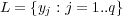 is the set of
  possible labels. This representation is shown in Table 1. Considering this scenario, the task of a multi-label learning algorithm is to generate a classifier
  that, given an unlabeled instance
  , is capable of accurately predicting its subset of labels
  , i.e.,
  , where
  is composed by the labels associated to the instance
  .
.
As stated earlier, in this work we use three multi-label methods which belong to the problem transformation category: Label Power Set (LP), Binary Relevance (BR), and BR+ (BRplus), an extension of BR we have proposed. It should be observed that methods from this category are algorithm independent. This is due to the fact that after transformation, any single-label learning algorithm can be used as a base-algorithm. A description of these three methods follows.
2.1 Label Power Set
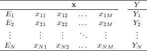
This method transforms the multi-label problem into one single-label multi-class classification problem, where the possible values for the transformed class attribute is the set of distinct unique subsets of labels present in the original training data. Table 2 illustrates this idea, where the attribute space was omitted, since the transformation process only modifies the label space. The first table shows a multi-label set of instances in the original form, while the second table shows the same set of instances transformed into the Label Power Set format, where notation  means that the respective instance is labeled with the conjunction
  . Observe that in the first table the set of labels
  is
is  while after transformation, the set of multi-class labels is
 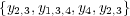 .
.

Using this method, learning from multi-label examples corresponds to finding a mapping from the space of features to the space of label sets, i.e., the power set of all labels, resulting in up to  transformed labels. Thus, although LP takes into account label dependency, when a large or even moderate number of labels are considered, the task of multi-class learning the label power sets would become rather challenging due to the tremendous (exponential) number of possible label sets. This is a drawback of the LP method. Another rather important issue is the class imbalance problem, which occurs when there are classes in the training set represented by very few examples. As the number of possible label sets increases with
  , this is likely to occur.
2.2 Binary Relevance
The Binary Relevance method is a problem transformation strategy that decomposes a multi-label classification problem into several distinct single-label binary classification problems, one for each of the  labels in the set
  . The BR approach initially transforms the original multi-label training dataset into
  binary datasets
  ,
,  , where each
  contains all examples of the original multi-label dataset, but with a single positive or negative label related to the single label
  according to the true label subset associated with the example, i.e., positive if the label set contains label
  and negative otherwise. After the multi-label data has been transformed, a set of
  binary classifiers
  is constructed using the respective training dataset
  . In other words, the BR approach initially constructs a set of
  classifiers — Equation 1:
 | (1) |
To illustrate the basic idea of the Binary Relevance transformation process, consider Table 3 which shows the four binary datasets constructed after the transformation (as stated before, since only the label space is used during the transformation process, the attribute space is not shown) of the multi-label dataset presented in Table 2. The possible values for the class attribute is “present” (or positive) or “not present” (or negative), denoted respectively by  and
and  .
.


To classify a new multi-label instance, BR outputs the aggregation of the labels positively predicted by all the independent binary classifiers.
A relevant advantage of the BR approach is its low computational complexity compared with other multi-label methods. For a constant number of examples, BR scales linearly with size  of the label set
  . Considering that the complexity of the base-classifiers is bound to
  , the complexity of BR is
  . Thus, the BR approach is quite appropriate for not very large
  . Nevertheless, as a large number of labels can be found in various domains, some divide-and-conquer methods have been proposed to organize labels into a tree-shaped hierarchy where it is possible to deal with a much smaller set of labels compared to
  [12].
[12].
However, the BR method has a strong limitation regarding the use of label relationship information. As stated before, BR fails to consider label dependency, as it makes the strong assumption of label independency. The BR+ method, explained next, attempts to diminish this limitation by trying to discover label dependency.
2.3 BR+
It should be observed that BR+ does not make any attempt to discover label dependency in advance. The main idea of BR+ is to increment the feature space of the binary classifiers to let them discover by themselves existing label dependency.
In the training phase, BR+ works in a similar manner to BR, i.e.,  binary classifiers are generated, one for each label
  . However, there is a difference related to the
  binary datasets used to generate the binary classifiers. In BR+, the feature space of these datasets is incremented with
  features, which correspond to the other labels in the multi-label dataset. In other words, each
  binary training dataset is augmented with
  binary features where
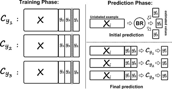
  . Figure 1, Training Phase, illustrates the binary datasets generated using a simple multi-label dataset with
  . After this transformation, BR+ constructs a set of
  binary classifiers to classify new examples in this augmented feature space — Equation 2.
 | (2) |
The classification of a new example could be carried out in a similar way to the standard BR approach using these augmented binary classifiers. However, as each one of these classifiers has been generated using a feature space which is different to the original one, the unlabeled examples must also consider this augmented feature space. In other words, the feature space of the unlabeled examples must be augmented accordingly to the training set that generated the corresponding classifier.
 .
.
At this point, BR+ is faced with the following problem: The feature space of the unlabeled examples is different to the feature space of the training examples used to build the binary classifiers.
To solve this problem, it is necessary to apply the same transformation process used with the training examples to the unlabeled examples. To this end, the set of unlabeled examples is also replicated, resulting in  unlabeled set of examples with the corresponding feature space for each of the binary classifiers generated in the training phase. On top of that, the value of those new features for the unlabeled examples are unknown, which leads to another problem:
How to estimate the values of the augmented features of unlabeled examples?.
In this paper, the values of the new features are estimated by BR+ in an intermediate step, where all the augmented feature values of unlabeled examples are initially predicted by BR (Initial Prediction in Figure 1) considering the original training data. The values predicted by BR are used by BR+ to complete the augmented feature space of the unlabeled examples. After this transformation, the unlabeled examples are classified by BR+ in a similar way to the standard BR method, considering all the original features plus the augmented ones for each individual classifier. This prediction strategy, illustrated in Figure 1 (Final Prediction), is called  (No Update), since no modification is made to the initial estimates of the augmented features during the prediction phase.
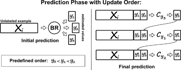
Furthermore, the BR+ method can use a different strategy to predict the final set of labels for unlabeled examples, where the values of the initial prediction for the augmented features are updated with the prediction of the individual binary classifiers as the new predictions are obtained, considering a specific order of classification — Figure 2.
 .
.
For example, if a predefined order to predict the individual labels is considered, each of the new values  can be used to update the previous value
  (initial prediction) of the corresponding augmented features of the unlabeled example.
To illustrate, consider as a predefined order the frequency of single labels in the training set, where the least frequent labels are predicted first, and consequently, updated first. We call this ordering, which does not depend on the classifiers, Stat (Static Order). Another possible order takes into account the confidence of the initial prediction for each independent single label given by BR, where labels predicted with less confidence are predicted and updated first in the final prediction phase of BR+. We call this ordering Dyn (Dynamic Order). Figure 2 illustrates the update process considering a predefined order (Stat).
Regarding BR+ computational complexity, it can be observed that it simply duplicates BR complexity. Thus, BR+ also scales linearly with the size  of the label set
  . Therefore, it is appropriate for a not very large
  .
.
3 Evaluation Measures
Evaluation measures usually used in single-label classification tasks consider only two possible states for an instance regarding its classification: correct or incorrect. However, in multi-label tasks, an instance can be classified as partially correct. Therefore, multi-label classification problems require different metrics than the ones traditionally used in single-label classification. Some of the measures used in the multi-label context are adaptations of those used in the single-label context, while others were specifically defined for multi-label tasks. A complete discussion on the performance measures for multi-label classification is out of the scope of this paper, and can be found in [13]. In what follows, we show the measures used in this work to evaluate the three multi-label classification methods considered. These measures are based on the average differences of the true set  and the predicted set of labels
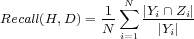
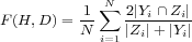
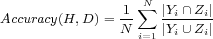
  , and are called example-based measures. The measures are Hamming Loss, Precision, Recall, F-Measure, Accuracy, and SubsetAccuracy, defined by Equations 3 to 8 respectively.
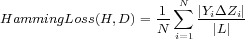 | (3) |
where  represents the symmetric difference between the set of true labels
  and the set of predicted labels
  . When considering the Hamming Loss as the performance measure, the smaller the value, the better the algorithm performance is, with a lower bound equal to zero. For the next measures, greater values indicate better performance.
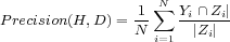 | (4) |
 | (5) |
 | (6) |
 | (7) |
 | (8) |
where  (true) = 1 and
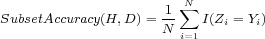
  (false) = 0. It should be observed that SubsetAccuracy is a very strict evaluation measure as it requires an exact match of the predicted and the true set of labels.
4 Experimental Set Up
A case study was carried out using unstructured data of medical findings related to the Upper Digestive Endoscopy tests. It follows a description of the original data, as well as the pre-processing carried out to obtain the corresponding multi-label dataset.
4.1 Case Study
Gastroduodenal peptic diseases, such as ulcers and gastritis, characterize a frequent pathological entity in the population. Upper Digestive Endoscopy (UDE) is an important test for the diagnosis of these diseases. From this exam, a medical findings report with information about esophagus, stomach, duodenum and results of the exam is generated.
In this case study, a collection of 609 findings without patient identifications were used. These findings were collected by the Digestive Endoscopy Service of the Municipal Hospital of Paulinia, São Paulo state, Brazil, which were stored as plain text in digital media. Each medical finding consists of five sections: esophagus, stomach, duodenum, biopsy and conclusions (diagnosis) of the test. The first three sections, as well as the last one, are described in natural language (Portuguese), while the biopsy section is described by structured information.
In this work, stomach and duodenum information was used in order to predict the diagnosis related to these two sections. The information related to the diagnosis of the 609 findings were analyzed manually and mapped into five different classes, two directly related to the duodenum and three to the stomach. Thus, each finding is associated to one up to five labels. However, it is expected that the number of classes will increase after these findings are further analyzed by specialists.
Regarding the unstructured information of medical findings, it has been observed that medical findings present the two following characteristics:
- the information is described using controlled vocabulary;
- the information consists of simple assertive sentences.
These characteristics were explored in [6] to extract/construct relevant attributes in order to transform the non-structured information of medical findings, described in natural language (Portuguese), to the attribute-value format.
In this work, we use a simpler approach to transform the unstructured information of the stomach and duodenum medical findings into an attribute-value representation than the one used in [6]. To this end, we used PreTexT 2 , a locally-developed text pre-processing tool, which efficiently decomposes text into words (stems) using the bag-of-words approach. It also has facilities to reduce the dimensionality of the final representation using the well known Zipf s law and Luhn cut-offs, as well as by ignoring user defined stopwords [16]. PreTexT 2 is based on the Porter
 s stemming algorithm for the English language, which was adapted for Portuguese and Spanish.
In this work, we choose to represent terms as simple words (1-gram), which are represented by the stem (attribute name) of simple words. As attribute values we used the frequency of the correspondent stem. Moreover, the minimum Luhn cut-off was set to 6 (1% of the number of medical findings), and the maximum Luhn cut-off was left unbounded. This way, the initial number of attributes, 244, was reduced to 108 attributes.
Summing up, the final attribute-value multi-label table, which represents the 604 medical findings used in the experiments, contains 108 attributes and  labels.
4.2 Algorithms
BR+ was implemented using Mulan, a package of Java classes for multi-label classification based on Weka, a collection of machine learning algorithms for data mining tasks implemented in Java. LP and BR are already implemented in Mulan. Furthermore, four base-algorithms, implemented in Weka and described in [17], were used in the experiments: (i) J48 (Decision Tree); (ii) Naïve Bayes (NB); (iii) k-Nearest-Neighbor (KNN); (iv) SMO (Support Vector Machines).
Preliminary experiments were carried out with  to determine the most appropriate
  value for KNN. The best results were obtained with
  , which was then used to execute KNN. Furthermore, the four base-algorithms were executed using default parameters.
5 Experimental Results
In this section, the performance of BR+ in the case study structured dataset is analyzed by means of comparison with LP and BR. All the reported results were obtained using 10-fold cross validation with paired folds, i.e., the same training and testing partitions were used by LP, BR and BR+ to obtain the average of the multi-label measures considered.
Table 4 shows the average of the example-based measure values described in Section 3. The numbers in brackets correspond to the standard deviation. For the sake of visualization, the best measure values are shown in bold. Arrow  indicates statistically significant degradation of LP or BR related to BR+. To this end, the Wilcoxon
 s signed rank test, a non-parametric statistical procedure for performing pairwise comparisons between two algorithms, was used.
Column BR+  shows the best possible results that could be obtained by BR+ using the corresponding base-algorithm. This value is obtained by a simple simulation which considers that BR+ always estimates the exact values of the augmented features of unlabeled examples during the Initial Prediction phase. In other words, the simulation considers
  — see Figure 1. Although we executed BR+ using the three different strategies
  ,
,  and
and  , we only show the results obtained using
  due to the fact that the three of them show similar results, and only in few cases
  and
and  show a slight degradation compared to
  . These few cases are commented in the text.
 indicates statistically significant degradation of LP ou BR related to BR+.
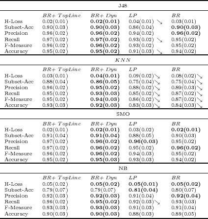
It follows an analysis considering each of the four base-algorithm used in the experiments.
- J48
- The measure values for BR+
 and BR+
  were the same as BR+
  , except for the Accuracy measure which was equal to 0.94(0.02) for both of them, slightly less than the Accuracy of BR+
  .
. As can be observed, BR+
 was able to obtain the top line values of BR+ in all measures using J48 as a base-algorithm. However, BR, which does not attempt to discover label dependency, also shows good results. As J48 generates a decision tree (DT) classifier, it has the flexibility of choosing different subsets of features at different internal nodes of the tree such that the feature subset chosen optimally, according to some criterium, discriminates among the classes in that node. In other words, DTs have an embedded feature selection, and only a subset of features are considered in the nodes of the tree. Thus, unless the augmented features of unlabeled examples are in the classification tree, the classification tree fails to discover labels dependency.
 Looking at the classification trees generated in each fold, it was observed that only in few cases the augmented features of unlabeled examples were part of the tree. This accounts for the slight improvement in some of the measures of BR+ over BR. It is worth observing that the participation of the augmented features of unlabeled examples in the tree classifier can be improved by attaching a positive weight to these features. This solution will be implemented and evaluated in the future.
Results using LP show that for J48 as the base-algorithm it is not competitive with BR+
 , and for three of the multi-label measures the results are significantly worse than BR+
  .
. - KNN
- The measure values for BR+
 and BR+
  were the same as BR+
  , except for the F Measure which was equal to 0.93(0.03) and 0.93(0.02) respectively, slightly less than the F Measure of BR+
  .
. Unlike J48,
 is a lazy learning algorithm which takes into account all feature values of the training set to classify an example. This characteristic enhances the properties of BR+
  . As can be observed, all measures for LP and BR are significantly worse than for BR+
  . Furthermore, all measure values obtained by BR+
  are near the BR+
  values.
 - SMO
- The measure values for BR+
 and BR+
  were the same as BR+
  .
. SMO is a support vector machine algorithm. This family of algorithms manage to construct a decision boundary (maximum margin separator) with the largest possible distance to the example points. This sort of decision boundary helps them generalize well. For example, it can be observed that LP, although not better than BR+
 , obtained its best results using SMO as the base-algorithm. As in the previous cases, BR+
  obtained the highest values for all measures, although none of them is significantly better.
 - NB
- Naïve Bayes uses Bayes theorem but does not take into account dependencies that may exist among features.
The measure values for BR+
 was the same for BR+
  and BR+
  . Besides, BR+
  achieved the best result for all evaluation measures comparing with BR and LP, except for Subset Accuracy. Furthermore, it outperformed LP with statistic significance for the Recall measure.
Summing up, as expected, it is possible to observe the influence of the base-algorithm in all methods tested. Nevertheless, in all cases BR+  presented the best results, except the Subset Accuracy measure using NB as the base-algorithm. A point to consider is related to the difference of BR and BR+
  evaluation measures, as greater differences indicate a higher possibility of BR+ improvements in relation to BR. This is the case when
  is used as the base-learning algorithm in which BR+ outperformed BR, as well as LP, with statistical significance.
6 Conclusions and Future Work
In this work, three different problem transformation methods, which map the multi-label learning problem into one or more single-label problems were considered: LP, BR and BR+. The main objective of BR+, for us proposed and implemented, consists of exploring label dependency by only using the binary classifiers to discover and accurately predict label combinations. In this work, we used an improved implementation of BR+, where a simple simulation can be carried out to determine the best possible results that BR+ can achieve in a dataset, enabling the user to narrow the search for the best base-algorithm for any specific dataset using BR+.
A case study using unstructured Upper Digestive Endoscopy medical findings, which were structured using the bag-of-words approach, was conducted. More specifically, stomach and duodenum information was considered in order to predict the diagnosis related to these two sections. It should be observed that medical findings have some specific properties and most conclusions are multi-label.
Previous experimental results on several benchmark datasets have shown the potential of the BR+ approach to improve the multi-label classification performance in datasets which do not have a very high label space dimensionality, as is the case of medical findings.
In this work, we used a simple approach to structure the natural language information of the medical findings used in the case study. As future work, we plan to structure the information using a more elaborated approach to extract/construct relevant attributes from medical findings, as the one described in [7], where a specific method to support the construction of an attribute-value table from semi-structured medical findings is proposed, in order to compare the power of both approaches.
However, the performance of multi-label classification depends on many factors which are hard to isolate. As future work, we plan to investigate further label dependency looking at the problem from different perspectives, in order to theoretically understand the reasons for improvements of the different measures used in multi-label classification.
Acknowledgements: This research was supported by the Brazilian Research Councils FAPESP and CNPq.
[1] Ethem Alpaydin. Introduction to Machine Learning. The MIT Press, 2nd edition, 2010.
[2] Matthew R Boutell, Jiebo Luo, Xxipeng Shen, and Christopher M Brown. Learning multi-label scene classification. Pattern Recognition, 37:1757–1771, 2004.
[3] Everton Alvares Cherman, Jean Metz, and Maria Carolina Monard. Métodos multirrótulo independentes de algoritmo: um estudo de caso. In Proceedings of the XXXVI Conferencia Latinoamericana de Informática (CLEI), pages 1–14, Asuncion, Paraguay, 2010.
[4] Everton Alvares Cherman, Jean Metz, and Maria Carolina Monard. A simple approach to incorporate label dependency in multi-label classification. In Proceedings of the Mexican International Conference on Artificial Intelligence (MICAI’2010)- Advances in Soft Computing, volume 6438 of LNCC, pages 33–43, Pachuca(MX), 2010. Springer-Verlag.
[5] Amanda Clare and Ross D. King. Knowledge discovery in multi-label phenotype data. In Proceedings of the 5th European Conference on Principles of Data Mining and Knowledge Discovery, pages 42–53, London, UK, 2001. Springer-Verlag.
[6] Daniel De Faveri Honorato. Metodologia de transformação de laudos médicos não estruturados e estruturados em uma representação atributo-valor, 2008. Master dissertation. University of São Paulo, Brasil. http://www.teses.usp.br/teses/disponiveis/55/55134/tde-10062008-154826/publico/dissertacaoDanielHonorato.pdf.
[7] Daniel Faveri Honorato, Maria Carolina Monard, Huei Diana Lee, and Wu Feng Chung. Uma abordagem de extração de terminología para construção de uma tabela atributo-valor a partir de documentos não-estruturados. In Proceedings of the XXXIV Conferencia Latinoamericana de Informatica, pages 1–10. SADIO, 2008.
[8] Tao Li, Chengliang Zhang, and Shenghuo Zhu. Empirical studies on multi-label classification. Proceedings of the 18th IEEE International Conference on Tools with Artificial Intelligence (ICTAI’06), pages 86–92, 2006.
[9] Tom M. Mitchell. Machine Learning. McGraw-Hill Education, 1997.
[10] Jesse Read, Bernhard Pfahringer, Geoffrey Holmes, and Eibe Frank. Classifier chains for multi-label classification. In Wray L. Buntine, Marko Grobelnik, Dunja Mladenic, and John Shawe-Taylor, editors, Proceedings of the ECML/PKDD, volume 5782 of Lecture Notes in Computer Science, pages 254–269. Springer, 2009.
[11] K. Trohidis, G. Tsoumakas, G. Kalliris, and I. Vlahavas. Multilabel classification of music into emotions. In Proceedings of the 9th International Conference on Music Information Retrieval, pages 325–330, 2008.
[12] G. Tsoumakas, I. Katakis, and I. Vlahavas. Effective and efficient multilabel classification in domains with large number of labels. In Proceedings of the ECML/PKDD 2008 Workshop on Mining Multidimensional Data (MMD’08), 2008.
[13] G. Tsoumakas, I. Katakis, and I. Vlahavas. Mining multi-label data. Data Mining and Knowledge Discovery Handbook, pages 1–19, 2009.
[14] Naonori Ueda and Kazumi Saito. Parametric mixture models for multi-labeled text. In Suzanna Becker, Sebastian Thrun, and Klaus Obermayer, editors, Proceedings of the NIPS, pages 721–728. MIT Press, 2002.
[15] C. Vens, J. Struyf, L. Schietgat, S. Džeroski, and H. Blockeel. Decision trees for hierarchical multi-label classification. Machine Learning, 73(2):185–214, 2008.
[16] Sholom Weiss, Nitin Indurkhya, Tong Zhang, and Fred Damerau. Text Mining: Predictive Methods for Analyzing Unstructured Information. SpringerVerlag, 2004.
[17] Ian Witten, Eibe Frank, Geoffrey Holmes, and Mark Hall. Data Mining: Practical Machine Learning Tools and Techniques. Morgan Kaufman Publishers Inc., San Francisco, California, EUA, 3 edition, 2011.
[18] Min-ling Zhang and Zhi-hua Zhou. Multi-Label learning by instance differentiation. In Proceedings of the Twenty-Second AAAI Conference on Artificial Intelligence, pages 669–674, Vancouver - Canada, 2007. AAAI Press.

