


 Inglés (pdf)
 Articulo en XML
 Referencias del artículo

 Permalink
1. Introduction
The province of Córdoba, Argentina, in the 20th century, had a consolidated wine industry with a national scope. However, it entered the 21st century having lost 90% of its capacity 1) and by the year 2023 it had an area planted with vines of 245 ha, 94% of which was used for wine production2. Understanding how the different pedoclimatic conditions present in the region interact with the vine and berry physiology and their impact on wine quality 3) provides useful information to those who must make decisions to reverse this situation. To identify and characterize these regions, the starting point is the zoning that can be done at the level of climate, soil and their interaction4. The role of climate is fundamental in the assessment of risks associated with adverse weather conditions such as extreme heat and frost, whose level of damage is related to the phenological stage of the vine 5)(6) . Climatic zoning is important for assessing the suitability of a specific region for viticulture because it is largely responsible for the diversity found in terms of wine quality and typicity7.
Daytime and nighttime temperatures and solar radiation influence the evolution of grape components such as sugars 8)(9) , organic acids 10)(11) 12, phenolic compounds 13)(14) 15 and aromatic compounds12. Knowing and, eventually, regulating the water status at different phenological stages of the grapevine makes it possible to control the vegetative growth of the plant and the yield and concentration of phenolic compounds in the berry16.
In relation to phytosanitary risks, it is necessary to know the humidity and temperature conditions between veraison and harvest because of the negative impact on the quality of grapes for winemaking as a result of cryptogamic diseases that can occur 17)(18) .
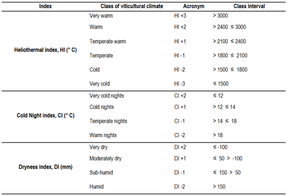
Specific bioclimatic indices have been created to determine the viticultural climate of the region. The most commonly used indices3 are the Huglin Heliothermal Index (HI)19, the Night Cold Index (CI)20, and the Dryness Index (DI) 20)(21) . The application of these indices allowed us to understand the spatial variation in viticultural potentialities and constraints in Uruguay17, Australia18, the United States22, New Zealand23 and France24.
Generally, bioclimatic indices are calculated and mapped using statistical methods from data collected as point samples whose distribution is rarely designed to capture climatic variability within a region. For example, available spatial information on air temperature is often limited, especially in sparsely populated or underdeveloped regions25. Air temperature values at unmeasured points can be predicted using interpolation methods based on measurements at meteorological stations. However, their accuracy is affected by arbitrary locations. These methods have proven successful in estimating air temperatures at locations close to meteorological stations26. The need for this spatial information has motivated some researchers to search for methods based on satellite information as a solution to this problem25. Thermal remote sensing data, such as Land Surface Temperature (LST), with high temporal resolution are an alternative because they can be estimated directly from remotely sensed radiance data27. Air temperature estimation using LST data has been applied in Africa25, Southeast Asia28, and Cordoba (Argentina)29. When calculating the differences in bioclimatic indices between air temperature and LST, the latter tended to have higher values at all spatial resolutions and showed a positive Pearson correlation with air temperature24. In regions with few weather stations, satellite data is a viable alternative for the estimation of Potential Evapotranspiration (Eto)30 and precipitation (pp)31, which has high spatio-temporal variability.
Geographic Information Systems (GIS)32 offer a robust platform for processing large volumes of spatial and temporal data needed for viticultural climate classification. Furthermore, the spatial visualization of data through GIS-generated maps facilitates not only the interpretation of the results by the scientific community but also their practical application by viticulturists and decision-makers.
The objective of this work is to identify and characterize regions with similar viticultural climates in the Sierras Pampeanas Cordobesas, which is useful information for managing viticultural practices, planting new vineyards and optimizing decision making in the face of changing trends in the viticultural climate of each region.
2. Materials and Methods
2.1 Description of the Study Area
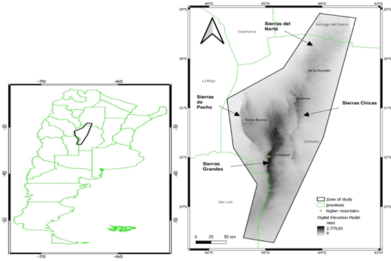
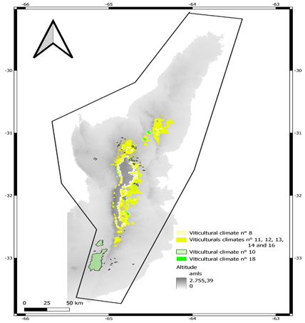
The study area covers an area of 50,062 km2 and is located in the west of the province of Córdoba (Argentina), including the entirety of Sierras Pampeanas Cordobesas (Figure 1). Seventy percent of its surface is steep, with differences between its western slopes, which are short and abrupt, and its eastern slopes, which have a greater areal extension and lower topographic gradient. The main mountain ranges that form them have a north-south orientation and are the Sierras Grandes (Cerro Champaqui: 2790 m), Sierras Chicas (Cerro Uritorco: 1950 m), Sierras de Pocho (Volcán Yerba Buena: 1600 m) and Sierras del Norte (Cerro de la Hoyada: 1056 m). Numerous intermountain valleys were formed between them.
The presence of the Sierras Pampeanas Cordobesas establishes a boundary between a subtropical monsoon climate in the center of the province of Córdoba and a warm semi-arid climate to the west of the Sierras. Intraserran climatic variation is dominated by an increase in altitude, which causes a decrease in mean air temperature33 of 0.5 °C for every 100 m increase in altitude. Therefore, there are regions with subtropical high altitudes and cold semiarid climates at altitudinal extremes34.
2.2 Satellite Data
The LST data and ETo were obtained from Moderate Resolution Imaging Spectroradiometer (MODIS), considered the most suitable sources because they are freely available and a very high temporal resolution of up to four observations per day during the day and night35. The MODIS sensor is onboard the TERRA or EOS-AM satellites launched in December 1999, and AQUA or EOS-PM launched in May 2002. The orbits of both platforms are helio-synchronous and quasi-polar with an inclination of 98.2° and 98°, and mean altitudes of 708 and 705 km, respectively. Both have a spatial resolution of approximately 1000 m in Bands 31 and 32, whose band centers are 10.78 and 12.27 µm and correspond to the far infrared or thermal. The MODIS products and their characteristics are listed in Table 1.
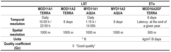
The algorithm used to obtain ETo is based on the logic of the Penman-Monteith equation and expresses the total potential water lost by evapotranspiration over eight days in kg/m 2(30) .
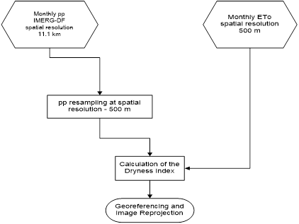
Precipitation values were obtained from the Integrated Multi-satellite Retrievals for Global Precipitation Measurement (IMERG) satellite products that provide quasi-global (60°N - 60°S) pp estimates from the combined use of passive microwave and infrared satellites that are part of the GPM constellation. The IMERG-F (IMERG Final) product has a daily and special temporal resolution of 0.1°, and the results were compared with monthly rain gauge data31.
Because pp and ETo are part of the same monthly water balance (Eq. 3), it is necessary for them to have the same spatial resolution. Therefore, resampling was performed, presenting the pp data in an image with the same number of pixels as ETo, which was 500 m.
2.3 Bioclimatic Indices Calculated from Satellite Data
Bioclimatic indices are indicators of the environmental conditions of a region and allow us to understand how climatic conditions influence vine growth and ripening. In this sense, in this paper, we chose to carry out an exploratory analysis of the different bioclimatic indices, presenting their spatial distribution and their interannual variation.
HI, CI, DI, risk associated with extreme temperatures and cryptogamic diseases between 2002 and 2022 were calculated. To obtain the different indices from the satellite images, Python scripts were used using the Rasterio library v. 1.3.1136.
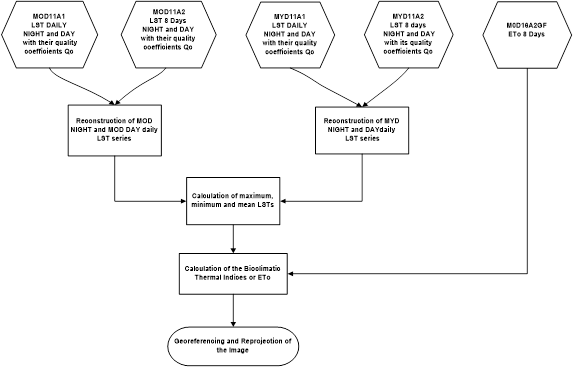
The data flow diagram for the estimation of the Thermal and Dryness Indices is presented in Figure 2 and Figure 3.
2.3.1 Heliothermal Index
Heliothermal Index was calculated with temperature records from September 15 to March 15 using Eq. 1:

Where
“d” is the long day coefficient whose value varies according to the latitude; for the study area a value of 1 was used.
LSTmed is the mean daily land surface temperature.
LSTmax is the maximum daily land surface temperature.
Four sets of daily LST data were obtained for each day. Daily LST images were downloaded using the M*DA11A1 and M*D11A2 daily and 8-day LST products, respectively, along with the quality values associated with each image. Only LST data “good quality” were used because they show better results in air temperature estimation35. MODIS data were collected from the USGS Land Processes Distributed Active Archive Center (LP DAAC) in HDF format. Missing or low-quality images owing to cloud cover were replaced by the values of the MYD11A2 and/or MOD11A2 products to create the daily LST time series. Using this methodology, extrapolation is avoided as a tool for estimating the missing data in the reconstruction of the temporal window24.
The Minimum LST value for each day was obtained from the MYD11A1 Night (1:15 h) product images averaged over MOD11A1 Day (10:08 h)24. This combination of MODIS products shows a better correlation with respect to Minimum Air Temperature because the lowest air temperature occurs in that time range35. The maximum LST value for each day was obtained from the MYD11A1 Day (14:00 h) product images averaged over MOD11A1 Night (22:50 h)24. The results of the evaluation of the influence of the overflight time on the air temperature estimation show that the proposed combination of MYDD-MODN images presents better correlation and justifies these results by the incorporation of the MODN product, which is night (22:50 h approx.); therefore its measurement is not influenced by solar radiation35. The mean LST value was obtained by averaging the maximum and minimum LST values for each day. These images were processed by a Python script in such a way that those pixels with Qc different from 0 were replaced by the value of their corresponding pixel of the temporally closest 8-day average product.
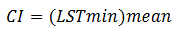
2.3.2 Cold Night Index
The LSTminimum of each day between February 15 and March 15 was obtained by averaging the corrected daily images of MYDN and MODN to subsequently calculate the average of the minimum LST of the aforementioned temporal period to obtain the CI according to Eq. 2. The latter was performed by means of a Python script which returns an image with the index values every 1 km2. As with the HI, it is geolocated and plotted according to the procedure described above.
2.3.3 Dryness Index
Dryness Index was calculated using Eq. 3 for the period Sep-15 to Mar-15.
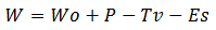
Where:
“W” is the estimated soil water reserve at the end of a given period (mm), which can be negative to express the potential water deficit but should not be greater than Wo.
“Wo” is the initial useful soil water reserve that can be accessed by roots (mm). A value of 100 mm was considered, which is the average value for the soils in the region37.
“P” is the pp (mm).
“Tv” is the potential transpiration (mm) in the vineyard calculated using Eq. 4:
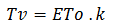
Where:
“ETo” is the potential evapotranspiration (monthly total in mm).
“k” is the coefficient of radiation absorption by the vine plant, which is related to transpiration and depends on its architecture and degree of development. The value of k should be adopted taking into account the month in which the water balance is being calculated, being 0.1 for September, 0.2 for October, 0.4 for November and 0.5 for the months from December to March20.
“Es” is the direct soil evaporation (mm), calculated using Eq. 5:
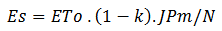
Where:
“N” is the number of days per month.
“JPm” is the number of days of effective soil evaporation per month and is calculated as the value of precipitation per month expressed in mm divided by 5; this value should be less than or equal to the number of days per month. Otherwise, the value of N is used.
2.3.4 Classes in Viticultural Climates
Each class of viticultural climate (Table 2) represents in addition to climatic differences the responses of the vine, grape or its products to those differences20, and was determined by processing in a Geographic Information System (QGIS v.3.28.11) the corresponding rasters of each of the bioclimatic indices as shown in the information flow diagrams in Figure 2 and Figure 3.
2.4 Climatic Risk Associated with Frost
The dates and geolocation where events of temperatures equal to or below 0 °C at the surface occurred were obtained by processing LST Night images of the MYDA11A1/A2 V.6.138 product from March 15 to May 15 for early frosts (EFD), and from September 1 to October 30 for late frosts (LFD).
2.5 Climate Risk Associated with Extreme Heat
It was calculated and geolocated by averaging the LSTmaximum obtained from the reconstruction of the daily series of the LST Day images of MOD11A1/A2 v6.1. and MYD11A1/A2 v6.1. products between February 15 and March 15.
2.6 Risk Associated with Cryptogamic Diseases
The pp value was estimated and geolocated for the period from February 1 to March 15.
2.7 Validation of the Results
To validate the climatic data obtained with remote sensors, a comparison was made with the records of two stations of the National Meteorological Service (SMN): Villa Dolores Airport and Cordoba Airport, the locations of which are shown in Table 3. This comparison was made by calculating the Pearson correlation coefficient and p-value between both series of the same index or meteorological variables.
3. Results
3.1 Integration, Grouping and Validation of Wine-Growing Climates and their Interannual Variation
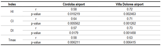
The integration of the three bioclimatic indices calculated, HI, CI and DI, makes it possible to determine and geolocate twenty climatic types (Table 4) which are grouped according to their climatic characteristics (Table 5), while the interannual variation is shown for the vineyard climates with the largest surface area of each group found. The Pearson's correlation coefficients and the p-value of the bioclimatic indices calculated with satellite data with respect to the NMS measurements at the two locations are shown in Table 6.
Table 4: Calculated values of DI, HI, CI, pp and maximum temperature (Tmax), LFD and TA (Thermal Amplitude) for each viticultural climate present in the study area with indication of the area it occupies
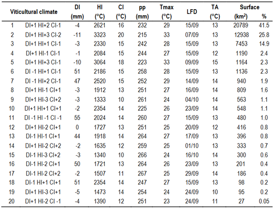
Table 5: r and p-values for the comparison of HI, CI, DI and Tmax calculated for two NMS stations with station data respect to satellite data
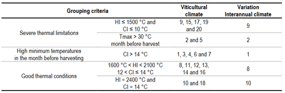
3.1.1 Regions with Viticultural Climates with Severe Thermal Constraints
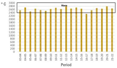
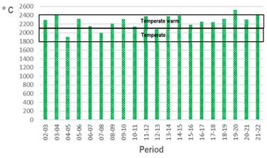
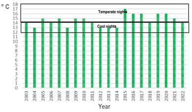
In this group it is possible to distinguish two different environmental conditions (Table 5). On the one hand, climates with mean maximum air temperatures above 30 °C in the month prior to harvest, and on the other hand, climates with very low temperatures located in the higher altitude regions. The territories included in the first subgroup have climates 2 and 5 (Table 4) occupying 28.2% of the total surface area (Figure 4). Wine-growing climate 2 shows an interannual variation in all the seasons analyzed of HI +3, CI -2 and maximum temperatures above 30 °C (Figure 5, Figure 6 and Figure 7, respectively). On the other hand, the vineyard climates 9, 15, 17, 19 and 20 (Table 4) occupy 2.3% of the area under study (Figure 4). The interannual variation of climate 9 shows in all seasons HI -3 and CI +2 (Figure 8 and Figure 9).
3.1.2 Regions with Viticultural Climates with High Minimum Temperatures in the Month before Harvesting
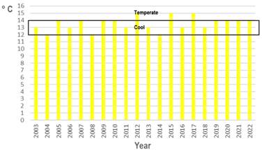
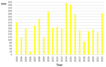
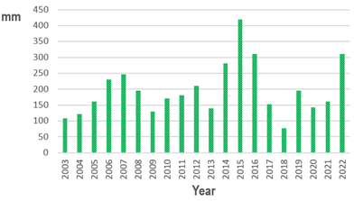
In an area that represented 62.9% of the study area, viticultural climates 1, 3, 4, 6 and 7 (Table 4) were identified (Figure 10). The interannual variation of Winegrowing Climate 1 shows values of HI +2, CI -1 and pp mostly below the average of 191 mm (Figure 11, Figure 12 and Figure 13, respectively).
3.1.3 Regions with Good Thermal Conditions for Wine Growing
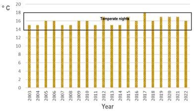
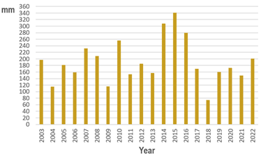
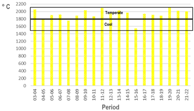
There are two different situations (Table 6 - Figure 14); on the one hand, regions presenting HI -1 and HI -2, and on the other hand, regions presenting HI +1. The territories included in the first subgroup have the winegrowing climates 8, 11, 12, 13, 14 and 16 occupying the 5.3% of the total area (Table 4). The viticultural climate 8 presents an interannual variation of HI -1, CI +1, pp mostly below average 206 mm (Figure 15, Figure 16 and Figure 17, respectively), and LFD 16/09; moreover, in the territories occupying 1.3% of the area under study the viticultural climates identified were 10 and 18 (Table 4). The interannual variation of winegrowing climate 10 shows HI +1, CI +1, and pp mostly below the average 197 mm (Figure 18, Figure 19 and Figure 20, respectively).
3.2 Water Balance
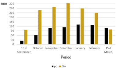
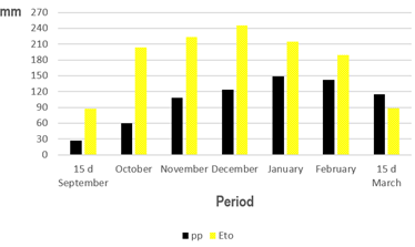
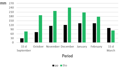
In the regions with viticultural climates 1, 8 and 10, which are the largest of the groups described in 3.1.2 and 3.1.3, the pp values were lower than ETo for the months of September, October and November (Figure 21, Figure 22 and Figure 23).
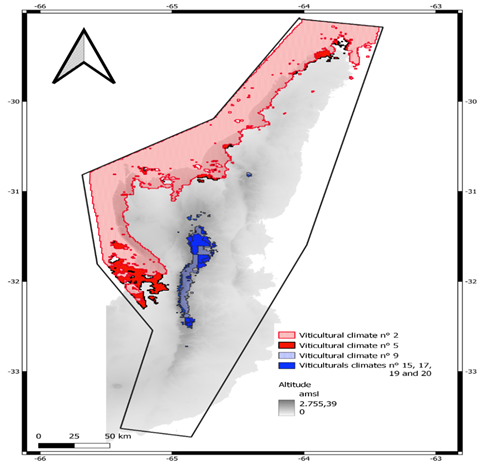
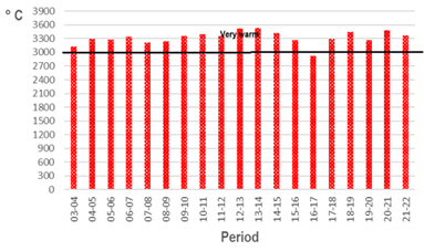
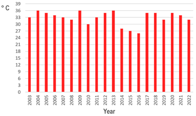
Figure 6: Interannual variation of the Tmax in the month prior to harvest for viticultural climate 2
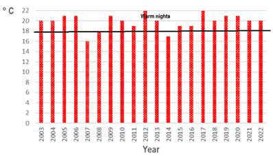
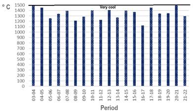
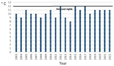
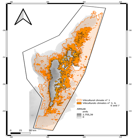
Figure 10: Regions with viticultural climates with high minimum temperatures in the month prior to harvesting
4. Discussion
The application of the SCCM for the identification of areas with different viticultural potential in the Sierras Pampeanas Cordobesas follows the methodology suggested by the OIV4. For the calculation of thermal indices, the daily LST MODIS series were used to replace air temperature. The comparisons made of LST MODIS with air temperature data at two SMN weather stations allow us to conclude that there is a significant linear correlation between them since the correlation coefficients calculated are significantly different from zero and the p-values found for all the data series compared were lower than the established significance level (α: 0.05), in coincidence with what was found in Vietnam35 and Africa25. Similar results were obtained for the HI comparisons, in agreement with those found in the Saint Emilion region (France)24. It was not possible to obtain correlation data for other locations due to the absence of meteorological stations in the study area.
With this methodology, it was possible to identify and delimit 20 zones with different homogeneous viticultural climates in the study region at the regional scale (Table 3), which could be grouped by common climatic conditions (Table 5) into three groups (3.1):
Areas with severe thermal limitations (Figure 4) exhibit two different antagonistic environmental conditions that affect the physiology of vines and berries in different ways. On the one hand, regions where, in the month prior to harvest, maximum temperatures exceed 30 °C, which leads to the assumption that berries and other plant tissues will reach temperatures above 35 °C39, conditions which produce a 50% decrease in total anthocyanins in Cabernet Sauvignon 13)(15) , in polyphenols in Tannat14 and in malic acid in the berry11; the photosynthetic apparatus of the leaves is affected9, as well as an increase in the respiratory activity, causing a higher vegetative growth of the plant at the expense of the growth and ripening of the berry, resulting in a net loss of assimilated carbon40. This thermal condition exhibited a similar behavior in the studied seasons (Figure 5, Figure 6 and Figure 7). On the other hand, higher altitude regions have heliothermic conditions in all the periods studied (Figure 8) that do not ensure berry ripening due to the specific requirements of the different varieties19. In addition, CI ≤ 10 °C (Figure 9) causes damage to plant tissues due to cold stress, affecting plant photosynthesis during daylight hours and affecting berry ripening9.
Regions with viticultural climates with high minimum temperatures in the month prior to harvesting (Figure 10), which presented CI -1, that reveal thermal conditions that do not favor anthocyanin synthesis and the preservation of aromatic terpene compounds in the berry 13)(20) . They do not present heliothermic limitations in terms of variety to be planted19, their maximum temperatures are lower than 30 °C and good TA and pp that indicate the risk of occurrence of cryptogamic diseases mainly during berry ripening 41) . The interannual variation of the viticultural climate 1 shows that this condition is maintained in all seasons (Figure 11, Figure 12 and Figure 13), so wines with limited chromatic and aromatic intensity are expected. In addition, it is necessary to primarily control Botrytis cynerea.
Among the regions with good thermal conditions for viticulture (Figure 14), it is possible to distinguish two different conditions: the first subgroup presents limited heliothermic potentialities (Figure 15) that require choice of varieties with requirements suitable to those conditions19, summer night temperatures optimal (Figure 16) for anthocyanin synthesis and preservation of mainly terpenic aromas, adequate TA; 40% of this territory presents DI -1 (Table 4), average pp (Figure 17) records that predispose to the development of fungal diseases41 and in line with what is expressed by Valdés-Gómez and others42, so it is necessary to carry out preventive viticultural practices to control this situation 43)(44) . The second subgroup does not present heliothermic restrictions19 (Figure 18), summer night temperatures (Figure 19) are suitable for the synthesis of polyphenols and the preservation of terpene aromas. Additionally, 85% of the area in this group is presented as DI +1 with pp records (Figure 20) that make it necessary to monitor vineyard health.
A water deficit is observed (Figure 21, Figure 22 and Figure 23) at a time when this situation is not advisable due to the phenological stage of the vines16, which indicates the need to irrigate.
In the region under study, the vines are between bud break and 10 cm buds (4 and 12 according to the Eichhorn and Lorenz45 scale) for the dates of LFD (Table 4). The more advanced the bud break, the more severe the frost damage to plant tissues, with consequent yield loss in the plant due to bud death or sprouting of secondary buds. Cabernet Sauvignon and Pinot Noir have little yield reduction because their secondary buds are fertile, but in the case of Riesling or Chardonnay, the yield reduction can be as high as 32%6. In these situations, in the planning stage of planting a vineyard, late budding varieties, plants with higher trunks, and plantings on high slopes should be considered because less frost damage is observed in vineyards planted in these locations46. For established vineyards, management techniques, such as delaying the pruning date to postpone bud break and thus avoiding exposing shoots to critical temperatures, or maintaining the soil by keeping it bare6 are recommend.
5. Conclusions
With this methodology it was possible to identify and characterize the viticultural climates of the Sierras Pampeanas Cordobesas, and it was possible to determine that 7% of the study area has no thermal limitations, while 63% has night temperatures above 14 °C, and the remaining 30% has severe thermal limitations. This information would allow the selection of suitable varieties for planting and the choice of viticultural practices in line with the environmental conditions of the regions that make up the area, and thus mitigate their adverse effects. Knowledge of this climatic suitability will allow the sustainable development of viticulture, considering that by periodically updating the information it will be possible to see how it varies in the context of climate change.
This work is intended to be part of a broader study that will address the confirmation of climatic differences in viticulture identified through surveys of the phenology of the vines planted there and the characterization of the wines obtained.
Despite the absence of meteorological stations and the size of the study area, the developed method allowed climatic zoning of the Sierras Pampeanas Cordobesas on a regional scale; thus, it would be feasible to apply it in other regions with similar characteristics. However, it is necessary to confirm local viticultural climates by conducting in situ studies.

