


 Inglés (pdf)
 Articulo en XML
 Referencias del artículo

 Permalink
1. Introduction
The use of whole-farm models to evaluate dairy production systems is suitable for estimating their biophysical, economic, social, and environmental performance. Whole-farm models are important tools for farm systems management and planning, and enable the evaluation of past, present, and future scenarios and the analysis of the national and global impacts of climate change, policies, or alternative technologies. More recently, the goal of whole-farm systems modeling is to help develop sustainable dairy production systems, including the wider societal benefit of more efficient production systems while reducing negative environmental impacts 1)(2) 3. In addition, whole-farm models can evaluate connections between system components that field research cannot empirically investigate, and provide information cheaper and faster than physical experimentation3.
In the Southern Cone (i.e., Uruguay, Argentina, Chile), the process of intensification of the dairy sector has been characterized in recent decades by increasing milk production per hectare, increasing stocking rate, supplying more concentrates, and improving the genetic merit of dairy cows 4)(5) 6. The dairy industries of this region have an increasing impact on the local and global economy, with the potential to increase milk production and comprise a great diversity of production systems7. However, economic performance alone will not determine the region's sustainability of pasture dairy production systems. In this context, the use of whole-farm models that allow visualizing the productive, economic, social, and environmental dimensions is necessary. Previous research has used different statistical analyses to calibrate, compare, or validate whole-farm models8. Suitable whole-farm models are needed within the Latin American region to simulate pasture dairy systems. Whole-farm models developed in New Zealand to simulate pasture dairy systems have been tested in Argentina9 and Uruguay10 using the annual results of farm systems studies. However, there is no data from whole farm models developed and tested in the region. A preliminary whole-farm model named “OLE! Dairy model” (OLE is an acronym for Organizador Lechero) has been recently developed for modeling specialized and dual-purpose farm dairy systems from the Latin America region. The unique aspect of this model is that it incorporates the biophysical, economic, social, and environmental dimensions of a dairy production system.
Statistical analysis is an important procedure during model calibration and evaluation, although there is no standard statistical approach11. Accuracy is the ability of the model to predict correct values, and precision is the model's ability to predict similar values consistently12. Assessing the adequacy of the model or its robustness is an essential step in the modeling process because it indicates the accuracy and precision of the model’s predictions12 by comparing the model results with actual data. The combination of several statistical analyses is essential to obtain representative statistical conclusions regarding the model's performance 11)(13) .
The objectives of the present study are (a) to describe the OLE! Dairy model for simulating the biophysical performance of pasture-based dairy production systems; (b) to evaluate the predictive capacity of the model with a set of statistical parameters, comparing its outputs with the biophysical performance of experimental dairy farm system studies, and (c) to calibrate by adjusting the technical coefficient.
2. Materials and methods
2.1 Model description
The OLE! Dairy model (version 2020 5.4) was developed by Francisco Candioti within the project named “Intensificación Sostenible de la Lechería” (LACTIS) funded by the Fondo Regional de Tecnología Agropecuaria (FONTAGRO). It works with Microsoft Excel 2010 or later and can be accessed with the link https://forms.gle/D9qyMk4NRJ9zsE9i8. The model is deterministic and uses a set of 12 sheets or screens accessed from the main menu, which refer to the biophysical, economic, environmental, and social components of the dairy production system. The present work will focus on describing and evaluating the biophysical component of the OLE! Dairy model.
The first versions of the model contemplated physical and economic aspects of the Argentine dairy systems. Within the framework of the LACTIS project, a team of dairy and livestock experts from the national research institutes of Latin American countries (Uruguay, Argentina, Costa Rica, Chile, Republican Dominican, Ecuador, Honduras, Nicaragua, Panamá, Paraguay, and Venezuela) was trained to use the OLE! and test it to simulate dairy or dual-purpose farm systems of their countries. This process involved workshops and meetings from 2018 to 2021 and yielded important modifications and improvements to the original model. Firstly, the model was adapted to heterogeneous milk production systems. As a result, very different systems can be simulated, from dual-purpose systems, typical of Central America, and specialized dairy production systems from the Southern Cone. Secondly, social and environmental indicators were added to be calculated from biophysical and economic inputs. The biophysical module of the model presents three main sections: (1) Feed supply, (2) Herd parameters, and (3) Herd composition and dynamics sub-model (Figure 1).
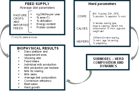
Figure 1: Flowchart of the OLE! Dairy model illustrating the major components of the biophysical module of the model and their interrelationships
2.1.1 Feed Supply
In this section, the information corresponding to the feed used in the production system to be simulated is entered. The feeds are categorized into three types: (i) perennial pastures: forage resources intended for direct grazing and reserves that last for more than one year; (ii) annual crops: annual forage resources intended for direct grazing and reserves, and (iii) bought-in feeds: concentrated and other feeds imported into the system. The following information must be provided for each feed: name of the feed, total production per hectare (kg DM/ha per year) for perennial and annual forage crops, and total amount (kg DM/ha per year) of imported feeds, % of the total livestock area occupied by each forage crop during its productive period, utilization (% of feed eaten by the animals), energy concentration (ME/kg DM), and crude protein concentration (CP; %DM). The main outputs regarding feed supply are total feed utilization efficiency (%), feed supply (kg DM/ha per year), average energy (ME/kg DM), and CP concentration (%) for total utilized feed.
2.1.2 Herd parameters
In this section, the information corresponding to the average herd parameters of the production system to be simulated is entered. Data must be entered for three different categories of animals based on the number of (i) adult cows, (ii) calves, and (iii) heifers.
Inputs for adult cows are the following: live weight (kg), milk protein content (%), milk fat content (%), lactation length (days), calving interval (days), abortions (%), rejection or cow sales (%), mortality (%). The ratio of milking cows to total cows (%) results from the relationship between the lactation length and the calving interval.
Inputs for calves are the following: proportion of females (%) (if sexed semen is used, values greater than 50% can be recorded), calves weaned (for specialized dairy systems, in this option, the daily liters supplied will have to be entered) or suckling (for dual-purpose dairy systems, in this option the daily hours of permanence of the calves with their mothers will have to be entered), days from weaning (days of milk consumption by calves), calf mortality (%). Data related to sales are also inputted: selling age (months), selling weight (kg), and proportion of young females for sale (%) (only in the case that part of the females are sold in early stages, which may be expected in dual-purpose production systems).
For heifers, the data required are the following: on-farm/off-farm rearing, mortality (%), age at first calving (months), and pregnancy efficiency in heifers (%).
2.1.3 Herd composition and dynamics sub-model
This sub-model generates a theoretical herd composed of milking cows, dry cows, and young categories as a result of the herd parameters entered by the user. In addition, it simulates its dynamics, calculating the meat sales of the different categories and the annual growth of the number of adult cows.
2.1.4 Biophysical outputs
The main biophysical outputs are proportion of the livestock area occupied by the adult herd (%) and young categories (%), stocking rate (cows/ha), individual production (L/cow per day), feed conversion efficiency (L/kg DM utilized), milk and milk solids productivity (L or kg MS/ha), milk consumed by calves (L/ha), feed intake (kg DM/cow per day), milk sales (L/ha) and meat sales (kg/ha) total, and for the different animal categories, theoretical adult herd growth (%). Theoretical adult herd growth (%) operates as an inventory difference that will have an impact on the economic result of the system. It can be positive (the number of replacement heifers exceeds the number of cows sold and culled) or negative (the number of replacement heifers is lower than the number of cows sold and culled).
2.2 Model calculations
The model calculates the quantity and quality of forage supply. For quantity, reference is made to three factors: Utilized Dry Matter (DM), Metabolizable Energy, and Crude Protein per average livestock hectare. For quality, the average diet is characterized by Energy Concentration (Mcal ME/kg DM) and Crude Protein (% CP).
The model estimates the proportions of livestock area occupied by adult cows and young categories. Then, it generates a theoretical herd based on the parameters entered by the user and estimates the energy requirements of the different categories. For this estimation, the model assumes that the ratio between the requirements of adult cows and the total requirements of the herd is equivalent to the ratio between the area of adult cows and the total livestock area.
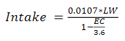
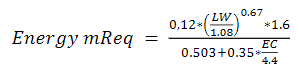
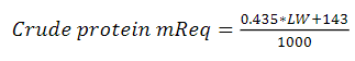
Intake (kg DM/milking cow per day) is calculated based on the cows' live weight (LW) and the quality of the average diet taking as a parameter the digestibility, which is calculated from the energy concentration (EC) (Eq. 1)14. The global energy (Eq. 2)15 and protein (Eq. 3)16 supply per cow is reached.
Energy (energy mReq; Mcal ME) and crude protein (CP mReq; Mcal ME) maintenance requirements are calculated, and the difference between energy/protein maintenance and energy/protein consumed is assigned to production.
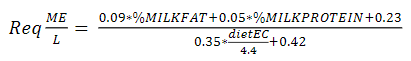
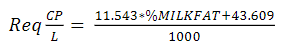
Taking the residual energy and protein values, the Individual Production possible by energy and by protein is calculated (Eq. 4 and Eq. 5) 15)(16) . The model takes as valid the lowest production value (Principle: law of the minimum).
Stocking rate (SR) is calculated by dividing utilized DM per hectare by individual intake, resulting in the number of cows per hectare for which the system achieves its balance between receptivity and SR (supply and demand) (Eq. 6)16. The model characterizes cows based on size and milk solids.
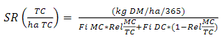
Where: MC= Milking Cows; TC=Total Cows; DC= Dry Cows; Rel= Relation; Fi= Feed intake
Dry cows and milking cows arise from the relationship between lactation length and interval between calving that comes from sheet 2. Milk Production per hectare is calculated by multiplying the Individual Production by the Stocking Rate per ratio of milked cow to total cow for 365 days.
2.3 Experimental description
The model was evaluated with data from a two-year farmlet experiment carried out in the Dairy Unit of the Experimental Station La Estanzuela of the National Institute of Agricultural Research (INIA), Colonia, Uruguay (34°20'S, 57°41'W). The farm description, pasture utilization, milk production, feed, and results are described in Stirling and others 10)(17) . The experiment consisted of a randomized complete block design with a 2×2 factorial arrangement. The experimental design resulted from the combination of two feeding strategies with different proportions of pasture in the diet: Grass Maximum (GMAX) or Grass Fixed (GFIX), and two cow genotypes: New Zealand (NZHF) or North American Holstein-Friesian (NAHF).
The four systems were designed to achieve the same annual production objectives: produce 1,000 kg of solids/ha and harvest 10,000 kg DM/ha per year of forage produced in the system (through pasture and mechanical cutting). The GMAX and GFIX feeding strategies aimed to reach different proportions of grazed herbage in the diet with the same level of concentrate supplementation per cow per year. Grass Fixed had pasture, concentrate, and silage allowance fixed at 1/3 each of the estimated annual total DMI, and all supplements were offered as a partial mixed ration on a feed pad. Grass Maximum had a flexible pasture allowance determined by pasture growth rate estimated weekly to maximize grazed herbage in the diet.
2.4 Statistical analysis
The model was evaluated by comparing the observed values from the farmlet experiment described above versus the simulated ones obtained from the OLE! Model. Data are for two consecutive years in each four treatments for eight observations. The following model outputs were evaluated: Individual Production (L/cow per day), Production per hectare (L/ha per year), Stocking Rate (cow/ha), and Total Intake (kg DMI/cow per day).
A range of model test parameters was calculated using the R18 statistical software, including:
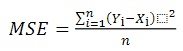
The Mean Squared Error (MSE), which is probably the most common and reliable estimate for measuring the predictive accuracy of a model12, and consists of the sum of the square of the differences between the observed (Yi) and simulated by the model (Xi), divided by the number of data (Eq. 7).
From this value, which is an absolute indicator (in the same units as the evaluation indicator), the result is relativized by the average or deviation of the observed values, leaving an indicator without magnitude.
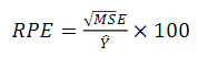
The Relative Prediction Error (RPE) is then calculated, which is expressed as a percentage from the square root of the MSE and the mean of the observed values (Eq. 8). This indicator is used to assess the goodness of fit between actual and predicted values, where RPE values <10% indicate that the model's predictions are good, values between 10 - 20% suggest reasonable predictions, and values >20% indicate mediocre predictions13.
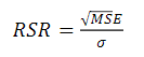
The square root of the MSE (RSR), but relative to the standard deviation of the observed values, (σ) is calculated to evaluate the error associated with the predictions of the model regarding the inherent variation in the observed values (Eq. 9). Values close to zero are considered better than positive values (<0.5, very good prediction; 0.5 - 0.75, good prediction; 0.75 - 1, moderate prediction; >1.0, the model needs improvements)19.
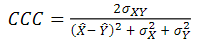
The Concordance Correlation Coefficient (CCC) was calculated as presented in (Eq. 10)20 using the R DescTools package21. The CCC combines measures of both precision and accuracy to determine how far the observed data deviate from the line of perfect concordance (diagonal). Lin's coefficient increases in value as a function of the nearness of the data's reduced major axis to the line of perfect concordance (the accuracy of the data) and of the tightness of the data about its reduced major axis (the precision of the data). Values of CCC near +1 indicate strong concordance between x and y, values near -1 indicate strong discordance, and values near zero indicate no concordance; there is no agreement on how to interpret other values.
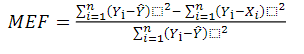
Model efficiency (MEF) was calculated according to Tedeschi12 (Eq. 11) as an indicator of goodness of fit, where MEF= 1 indicates perfect goodness of fit; MEF < 0 indicates that the values predicted by the model are worse than the observed mean.
2.5 Rapid calibration
In the herd parameters section, the only data that can be modified is the technical coefficient (default: 100%), an index that directly affects individual milk production. Its use is recommended in cases where a quick calibration of milk production is needed. To properly use the simulation model, it is advisable to first simulate the current known situation. This exercise allows the adjustment of inputs and results. In addition, it contributes to improving the understanding of the processes involved (diagnosis) and strengthens the baseline on which alternative scenarios can be simulated.
In its biophysical components, the OLE! model involves a large number of variables. In this framework of complexity, it may be that even after thoroughly reviewing the inputs, some small deviation persists in the results. To facilitate the adjustment specifically of individual production in the event of small deviations that cannot be explained, the model offers the possibility of changing the technical coefficient. It may eventually be corrected upward under controlled or in conditions of higher production levels than the average.
Once the baseline has been simulated, reviewed, and calibrated, alternative scenarios can be simulated by changing certain inputs (“what would happen if…?”). A large number of alternatives and combinations can be simulated in a short time without the cost or effort of putting them into practice. For example, in situations where individual milk production is limited, such as in extreme weather events, the index could be adjusted below 100%. On the other hand, in cases where the model may underestimate individual milk production, such as in the case of highly efficient milk production systems, the index could be increased above 100%. A calibration was carried out on the model to adjust the production per hectare of the simulated systems. To do this, the Individual Production coefficient was increased from 100 to 110%, improving the productive performance of milking cows.
3. Results
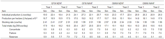
The observed values from the experimental study versus the simulated values using the OLE! Dairy model are detailed in Supplementary material (Table 1).
The model's predictive capacity was evaluated on the following variables: Individual Production (L/cow per day), Production per hectare (L/ha per year), Stocking Rate (cow/ha) and Total Intake (kg DMI/cow per day).
The model presented a good predictive capacity for Stocking Rate and concentrate, pasture, and reserve Intake (kg DM/cow per day) for the four systems evaluated during the two years (Table 2). The model's predictive capacity for Individual Production and Production per area was reasonable, as indicated by the RPE values <20% (Table 2); however, the RSR, CCC, and MEF showed values that represent deficiencies in the model for the prediction of these variables.
Table 2: Predictive capacity of the OLE! Dairy model for Individual Production, Production per hectare, Stocking Rate, Total Intake, Concentrate Intake, Pasture Intake, and Reserve Intake for the total data set (n = 8 observations)
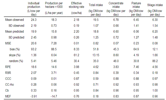
MSE, mean square error; RPE, relative prediction error (root mean square prediction error RMSPE/mean observed) ×100; RSR, ratio of RMSPE to standard deviation of observed values; CCC, concordance correlation coefficient; CC.rho, Correlation Coefficient; Cb, Bias correction factor (i.e., the line of perfect concordance); MEF, Model efficiency.
Figure 2a shows the Individual Production (Simulated X-axis, Observed Y-axis), where it is observed that the model underestimates Individual Production (L/cow per day); the grey circle and squares treatments that represent the North American breed Holstein-Friesian (NAHF) are separated from the treatments with black circles and black squares that represent the New Zealand breed (NZHF), this being associated with the breed's production factor.
Figure 2b shows the Production per hectare (Simulated X axis, Observed Y axis); however, a pattern is not shown as in Figure 2a since the model uses the weight of the animals as a variable for the calculation of the Stocking Rate, this indicator is used to calculate Production per hectare. The model presented a better fit concerning the observed in the experimental design for Individual Production (Figure 3a). For Production per hectare (Figure 3b), when increasing the Individual Production coefficient to 110%, the model did not present a characteristic pattern as observed in Figure 2a.
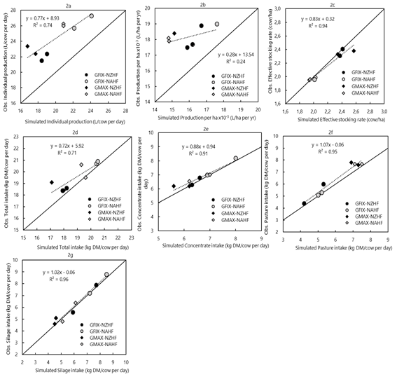
Figure 2: Relationship between observed and simulated for Individual Production (2a), Production per ha x 10-3 (2b), Stocking Rate (2c), Total Intake (2d), Concentrate Intake (2e), Pasture Intake (2f), Reserve Intake (2g ), for the four systems modeled during 2-year experimental period (2017-2018) for the total data set (n = 8 observations)
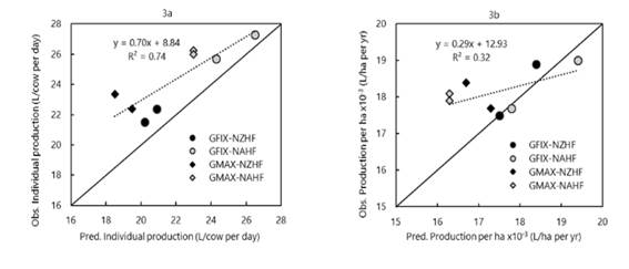
Figure 3: Relationship between observed and simulated for Individual Production (3a), and Production per ha x10-3 (L/ha per yr.) (3b), for the four systems modeled during 2-year experimental period (2017-2018) for the total data set (n = 8 observations)
The model presented a good predictive capacity for Individual Production (L/cow/day) and Production per hectare (L/ha per year) variables, with an increase of 110% (Table 3).
Table 3: Prediction capacity of the OLE! Dairy model increasing 110% the technical coefficient for Individual Production and Total Production for the total data set (n = 8 observations)
| Individual production (L/cow per day) 10% | Production per hectare ×1000 (L/ha per year) 10% | |
| Mean predicted | 21.98 | 17.45 |
| SD predicted | 2.70 | 1.08 |
| MSE | 7.35 | 1.83 |
| bias (%) | 76.91 | 47.72 |
| slope (%) | 8.05 | 30.81 |
| random (%) | 15.03 | 21.46 |
| RPE | 11.12 | 7.35 |
| RSR | 1.24 | 1.86 |
| CCC | 0.35 | 0.13 |
| CC.rho | 0.55 | 0.23 |
| Cb | 0.64 | 0.58 |
| MEF | -0.75 | -2.96 |
MSE, mean square error; RPE, relative prediction error (root mean square prediction error RMSPE/mean observed) ×100; RSR, ratio of RMSPE to standard deviation of observed values; CCC, concordance correlation coefficient; CC.rho, Correlation Coefficient; Cb, Bias correction factor (i.e., the line of perfect concordance); MEF, Model efficiency.
4. Discussion
The OLE! Dairy model has been tested in its biophysical component with a real database from dairy production systems located in the region's humid subtropical temperate climate zone. The database allowed us to understand the model's performance as it was tested in contrasting production systems over two years. The variability in the inputs was what generated the variability in the model’s predictions2.
Regardless of the experimental design, the model presented a good performance for total DM intake, for each diet component (concentrate, pastures, and reserves), and for the Stocking Rate, indicated by most statistical analyses (Table 2). In terms of individual milk production, the low fit between the model’s predictions and the observed data can be observed in the MSE, which is found at 20.7 (Table 2). This value is mainly explained by the high bias (93.2%), which indicates that the model systematically underestimates Individual Production, being able to observe that the data set is correlated but above the diagonal (Figure 2a). The MSE estimate is a reliable measure of the model's accuracy; however, the reliability will decrease as the number of observations decreases12. The MSE is made up of three components: the bias, the slope, and the randomness. The interpretation of these results can provide us with some indications of the possible causes of the lack of precision in the model13. For Individual Production, although there is a bias, the model fits in reasonable terms (RPE <20%) but shows a worse fit than the Stocking Rate and Total Intake (RPE <10%)13.
In the process of evaluating a model with independent data, as in this case, the bias is an indicator of the robustness of the model, while the slope is used to evaluate the presence of structural problems in the model 13)(22) . In the present study, the bias was greater than the slope and the randomness for Individual Production and Production per hectare variables, which implies that the model has low precision for these indicators. If we observe the RSR, it indicates that this value is greater than 1, which implies that the model requires improvement in this variable19, being a very good prediction for the Stocking Rate and the DM intake of each diet component (concentrate, pasture, and reserve), and a good prediction for daily total DM intake. Although the R2 is high (Figure 2a), the CCC for Individual Production shows a non-concordance explained by a high bias (Cb 0.33, Table 2). In the case of Stocking Rate and Total Intake, there is a high concordance between the simulated and observed values21.
The same occurs in the MEF, with Individual Production being a value that is far from 1 and negative, which again shows the underestimation of the model for this variable, given that the values predicted by the model are worse than the observed mean. For Total Intake and Stocking Rate, the MEF presents a very good goodness of fit12.
Production per hectare is the product of Individual Production and the Stocking Rate, which presented a low general fit in the statistics. This is explained in part by the aforementioned Individual Production bias problems. However, it is also shown that, depending on the experimental design, the simulated data generated a low R2 (Figure 2b), explained by the effect of an increase in the Stocking Rate due to the weight of the animals and the effect of higher production associated with the animal genotype, magnifying the negative adjustment in the statistics made.
The model underestimates the observed values because Individual Production is deducted from the Total Intake of energy/protein nutrients by the value corresponding to maintenance, assuming that the remaining balance is used for production. The maintenance equation takes the fasting metabolism as a base and weights it by an increasing factor (i.e., 1.6). This increase factor is associated with different factors such as energy expenditure in pasture, walking, and energy loss due to heat or other means (Eq. 2). This difference is more noticeable in the experimental case. However, in commercial farms, these values have been much more precise, which may be due to the fact that the experimental designs use few animals, a homogeneous control of herd management, feeding conditions, and environmental factors; unlike commercial systems, which tend to have greater individual differences in large herds as well as differences in management, feeding and environment.
Total Intake is affected by digestibility. Cows within the treatment with greater inclusion of pasture generated greater uncertainties. With a greater supply of pasture, the animals may have a greater selection, resulting in a greater digestibility (energy concentration) of what is consumed. This actual digestibility is greater than the one put into the feed inputs, generating greater total energy consumption, and consequently, greater Individual Production than that which would be estimated from the average value. This consumption is greatly affected by the amount of forage available, the original structure of the pasture, organic matter content and digestibility of the pasture, NDF, and the pasture 23)(24) 25.
The underestimation could have a substitution effect with the addition, probably due to the possibility of selecting a higher quality pasture, because they have a greater supply of pasture and an increase in the time dedicated to grazing25. The information needed to estimate intake in grazing cows is more complex and demanding. In addition, it is always advisable to check the feed quality inputs in terms of energy and protein concentration. If differences persist, the technical coefficient can be used as a rapid calibration tool.
When the technical coefficient was increased by 110% to increase the cow's Individual Production, the GFIX production systems fit much better but not so different from the GMAX production systems (Figure 3a and Figure 3b). The model presents a better predictive capacity by increasing the technical coefficient by 110%, both for Individual Production and per hectare (Table 3). This allows users of the model to have greater precision, considering the characteristics of the production system, to adjust or calibrate the model to their requirements, being a tool that was developed thinking about the diversity of production systems found in Latin America, covering intensive milk production systems or dual-purpose systems. In the case of production systems with a greater inclusion of grazing, this technical coefficient may be more useful than in systems with a fixed diet.
Although the model does not discriminate based on animal breed or biotype, the difference between both treatments is reflected in the Stocking Rate within the experimental design (Figure 2c). This is reflected in the grey circles and squares treatments that represent the North American breed Holstein-Friesian (NAHF), which are separated from the treatments with black circles and black squares, which represent the New Zealand breed (NZHF). This is due to the animals’ body weight as the main characteristic. The model has good accuracy for the statistical analyses performed (Table 2).
In models that share other indicators such as economic, social and environmental, this underestimation would generate erroneously high predictions. On the contrary, the overestimation could result in more conservative decisions, and the alternatives evaluated as profitable could be more favorable than expected13.
5. Conclusions
We were able to test the model in its biophysical component, which is a model of great help for the planning and management of dairy production systems that can be used in the Latin American region. The model presented a good statistical adjustment to the Stocking Rate and Total Intake variables. However, the Individual milk production and Production per hectare variables could have presented a better statistical fit. The ability of the model to perform a rapid calibration allows for avoiding overestimation or underestimation that generate erroneous measurements in the planning and management of milk production systems, being able to adjust to the different production conditions of the region.