Keywords: volume segmentation, GrabCut, flow network, minimum cut, Push-Relabel.

Spanish keywords: Segmentación de volúmenes, GrabCut, red de flujo, corte mínimo, Push-Relabel

Received 2012-05-30, Revised 2013-01-15, Accepted 2013-01-15

1 Introduction

The image segmentation is a process that consists in separating an image into two or more different regions. Each region is homogeneous in accordance with some similarity criteria predefined. When the image represents a volume (3D image), the process is called volume segmentation.

There are several approaches to perform a volume segmentation, though these algorithms require a significant processing time (1, 2). Recently, a set of algorithms on the GPU (Graphics Processing Unit) have been developed to exploit their native parallelism, and obtain better time results than traditional algorithms executed in the CPU. Noticeable examples of these algorithms are developed in the CUDA (Compute Unified Device Architecture) developed by Nvidia (3). It provides a parallel computing architecture to make algorithms to be executed on multiples cores on the GPU.

Volume segmentation algorithms are highlighted between the algorithms executed using the GPU. Especially in the field of medicine, the segmentation takes an important role. Thus, when is necessary to extract a particular region to further medical diagnosis, volume segmentation is totally required.

In this paper, we present an approach based on the GrabCut algorithm developed by Rother et al. (4), for the volume segmentation using CUDA. Our contribution can be summarized as follow:

• An adaptation of the GrabCut algorithm to 3D image segmentation.
• A Push-Relabel maximum flow algorithm on the GPU.
• Introduction of some changes in the original formulation of the GrabCut algorithm.

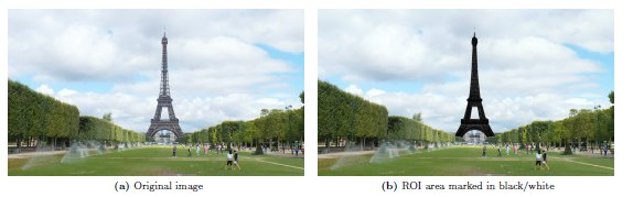
Using our approach, first the user must select a ROI (Region Of Interest) inside the volume to be segmented. In image context, a ROI is defined as a section inside the image which indicates the area to be processed using a certain algorithm(s), see Figure 1. Following, the algorithm is executed and returns two sub-volumes: foreground (region of interest) and background (remaining). The algorithm builds a flow network (5) based on the voxels color of the ROI (according to a transfer function). We created a parallel version of the algorithm Push-Relabel executed and stored on graphics hardware. At the same time, it provides a scheme for treatment of inactive threads on the GPU. Finally, results are studied and compared between two implementations of the same algorithm: CPU (sequential) versus the GPU (parallel).

This paper is organized as follow: Section 2 presents an introduction to the area of segmentation as a graph problem. Section 3 describes previous works in the area. Following that, in Section 4, we explain details of our proposal to the volume segmentation. Next, in Section 5, experiments and performance, qualitative and memory consumption results are presented. Finally, conclusions and future works are presented in Section 6.

2 Segmentation Based on Graph Algorithms

Several problems on image processing can be expressed in terms of energy minimization. In recent years, max flow minimum cut algorithms have emerge as tools for precise or approximate energy minimization (6). The idea consists in representing each pixel of the image as a graph node (using a pixel labeling approach), and connect each node with others using weighted edges. Then with this built graph, an energy function is applied with a minimal cut algorithm on the graph, which also minimizes energy. This statement was proposed by Greig et al. (7) in 1989. With this, the minimal cut process in a graph can be computed efficiently by a maximum flow algorithm.

In 2001, Boykov et al. (8) develop an approximation to the minimization of energy based on a representation of the image as a graph. Following, Boykov and Kolmogorov (9) present an experimental comparison of the efficiency of min-cut/max-flow algorithms for segmentation. Several types of image features are considered to separate two components under energy minimization: color, gradient values, similarity and so on.

In graph theory, it is possible to define a graph as which contains a set of nodes and edges. A cut is defined as a partition of a graph into two disjoint subsets. It is performed eliminating the set of edges to obtain two subgraphs and such as . A cut has a weight obtained as a sum of all weights of edges removed, . In a graph, there are several ways to obtain a cut. Furthermore, the minimal cut is the cut with the smallest weight of all possible cuts in the graph.

Following the min-cut/max-flow theorem (5), the minimal cut in a graph can be performed executing a max-flow algorithm. A max-flow algorithm consists in determining the maximum network flow that goes through a source node and reaches a target node. Thus, the saturated edges (edges with ) are eliminated by the algorithm to obtain the minimal cut. Among the most used algorithms to compute the minimal cut, there are those proposed by Ford and Fulkerson (10) and the ones proposed by Goldberg and Tarjan (11) called Push-Relabel. A remarkable technique where the min-cut/max-flow is implemented efficiently, is called GraphCut (12).

Based on the GraphCut algorithm, Rother et al. (4) introduce a novel approach named GrabCut, where a graph is divided into two regions using the min-cut/max-flow theorem: background and foreground. An energy minimization function based on color similarity is applied to reach the segmentation. The next section presents a subset of notable works on volume segmentation area, focusing on the GrabCut.

3 Related Works

In literature, exist many algorithms of volume segmentation. In recent years, algorithms based on image-graph representations, which assign statistical values on weight edges and separate the graph on ROIs have considerable grown. Thus, there are several graph based approaches for image segmentation. Specifically, the GraphCut algorithm proposed by Boykov and Jolly (12) applies a minimal cut algorithm over the built graph and splits it up into 2 regions (foreground and background). Based on that, Boykov and Funka-Lea (13) present a complete review of detailed technical description of different proposals that use the GraphCut algorithm for image segmentation. More recently, there are numerous research works (14, 15, 16, 17) based on the GraphCut approach which extend it to improve the segmentation process in different scenarios. A notable work which uses the GraphCut approach is the GrabCut algorithm. In 2004, GrabCut was introduced by Rother et al. (4). An example of the implementation of the original GrabCut algorithm over a particular problem is presented in (18) where tumors are segmented using endoscopic images.

Puranik and Krishnan (19) present a complete and recent survey of volume segmentation algorithms for medical images which exist in the literature. In that work, they show a brief classification of segmentation algorithms in structural, statistical and hybrid techniques. In 2012, there is a significant research presented by Santle and Govindan in (20) which shows a complete review of segmentation based on image-graph algorithms.

Nowadays, there are techniques which execute algorithms on the GPU (21, 22, 23) to accelerate the volume segmentation process. In 2005, Schenke et al. (24) reviewed the GPU algorithms and classified them into pixel-based methods, edge-based methods and region-based methods. This classification is made according to the location where the segmentation process is applied. In the next section, we present our proposal to accomplish a volume segmentation based on GrabCut using GPU.

4 Approach

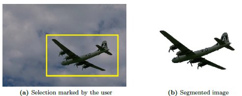
The GrabCut is an iterative and minimal user intervention algorithm, which combines statistical values based on the GraphCut algorithm (12) to separate an image in foreground and background. The input of the algorithm is an image and a region to segment. The region is defined by the user with a single rectangle. Figure 2a shows how the user selects a box (in yellow color) inside the image to indicate the region of interest. Figure 2b presents the results obtained after performing the GrabCut algorithm.

Our approach is an extension of the original 2D GrabCut to the 3D space. The algorithm requires the source volume and a sub-volume selected by the user. Then, the algorithm creates a flow network (5) where each voxel is a graph node. Each node is linked to its neighbors using weight edges called N-Links (the maximum number of neighbors is 26). In a flow network there are two special nodes: source and sink . The source is connected to each voxel inside the user selection to compose the foreground. Thus, the sink node is connected to each voxel outside the user selection to the background.

All nodes are connected to the source through weighted edges called T-Links. The weights are calculated using Gaussian Mixture Models (GMM) (25). The background and foreground groups are formed by gaussian components, with . Each gaussian component belongs to a GMM and it is derived from the color statistics in each region of the image. The aim is to separate components which contain a group of similar color voxels. For this purpose there are several techniques, particularly in this paper a color quantization technique developed by Orchard and Bouman (26) is used.

Once the graph is built, the min-cut algorithm must be applied. In the paper presented by Rother et al. (4), Ford-Fulkerson algorithm is used. In this proposal, we employ the Push-Relabel algorithm because it can be parallelized on the GPU. Thereby, once applied the min-cut, the graph is separated in foreground and background, and the process can be performed over again until all nodes are part of a group.

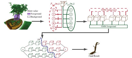
Figure 3 shows an overview of our approach. First, the user selects the ROI (purple color box). With this selection, a list of matte values are created and the N-Links are constructed. For each voxel, a matte value indicates to which group belongs (background or foreground). If a voxel is inside the user selection then it belongs to the matte foreground group. Otherwise, it belongs to the matte background group. These matte values are modified during the algorithm execution.

Figure 3: Steps of the proposed 3D volume segmentation.

Next, to each voxel a probability value is assigned belonging to each component of the GMM background and GMM foreground . This process is performed on all voxels in order to obtain the T-Links values. After the graph has been constructed, the minimal cut is achieved separating the graph in 2 sub-graphs. In Figure 3, these are represented by the green cubes to the foreground and red cubes to the background. The min-cut algorithm applied is based on a Push-Relabel approach (11) and fully implemented on the GPU. Finally, background voxels are removed to get the final result.

The following sections explain in detail the approach to obtain the value of N-Links, T-Links and the Push-Relabel algorithm.

4.1 N-Link

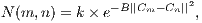
Between two nodes and , the N-Link value is computed assuming the distance between them is 1. Then, the formulation pesented by Mortensen and Barrett (27) is applied (equation 1).

(1)

where represents the euclidean distance in RGB color space to voxels and . The value is a constant that ensures a difference in distance between color values of voxels. The constant value is a suggested value in the work developed by Blake et al. (28) about the Gaussian Mixture Markov Random Field (GMMRF) model calculations. Equation 2 shows how to calculate , which is a variation of the original formula presented in (12).

(2)

The value of represents the number of voxels in the volume, and describes the number of neighbors to each voxel. In this proposal, every voxel has neighbors in directions , and . Then, the value of is except at borders which can take values from to .

As mentioned above, a N-Link connects a voxel with a neighbor voxel . Also, each voxel has to be connected to the foreground and background group through a link called T-Link. The next section presents how we calculate these T-Links.

4.2 T-Link

When the user selects a region to be segmented, voxels inside the selection are marked as unknown voxels, and those outside are marked as background voxels. On each iteration of the algorithm, it calculates the value of the GMM of every voxel and determines in which group a voxel belongs. Then, an unknown voxel can change its value to be part of the background or foreground group. These voxels connections are called T-Links.

Each voxel has a T-Link connected with the foreground, , and with the background . If a voxel belongs to the foreground then the min-cut does not disconnect it from this group. For that voxel, the condition can be guarantee assigning the value of the and , where represents the maximum possible weight of an edge. Similarly occurs if the voxel belongs to the background, i.e. and . Thereby, when a m-voxel is marked as unknown then and . The and indicate the probability of to belong to the GMM foreground and background respectively.

It is possible to define the probability of the m-voxel as:

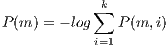(3)

where represents the number of component of the GMM. The value of is the probability of a m-voxel to belongs to a component . The computation of follows the method applied by Talbot and Xu (29). Aforementioned, in this paper there are five components used. Thus, to each voxel the value of and of all components must be calculated.

Once the values of N-Links and T-Links are calculated for all nodes, the Push-Relabel algorithm is applied to obtain a minimal cut. Next, we explain this algorithm in detail.

4.3 Push-Relabel

The Push-Relabel algorithm was proposed by Golberg and Tarjan (11) in 1986. It is an iterative algorithm to calculate a minimal cut in a graph, specifically in a flow network. In a flow network , there are two special nodes: source node and sink node . Additionally, the Push-Relabel algorithm constructs a residual graph which consists of a graph with the same topology of , but composed by edges that support more flow. A sent flow from a node to a node , , must be less or equal than the capacity of the edge between and , . The graph changes the weight of the edges (flow capacity) during the algorithm execution. It is possible to define the residual capacity as the amount of flow that can be sent from to , after sending . The residual capacity is computed as:

(4)

Basically, the algorithm stores two values: the flow excess and the height of each node. The value of indicates the difference between incoming flow and outgoing flow for a node . The height is an estimate value of the distance from to . At first, all nodes are , except the source node whose height is , where is the number of nodes in the graph. There are two basic operations in the algorithm: Push and Relabel. A Push operation from node to consists in sending a part of the excess from towards . To perform a Push operation, the following conditions must be satisfied:

1. ; it must exists a flow excess in .
2. ; it must be available capacity to sent flow from to .
3. ; the flow can only be sent to a lower height destination node.

Then, it is possible to derive that the flow sent is equal to .

In the Relabel operation, the is increased in 1 until it becomes greater than the height of all nodes to which the flow can be sent. The conditions for this operation are:

1. ; a flow excess in exist.
2. for each such that ; only the nodes with available capacity to send flow are considered.

Then, the increasing of the height is calculated as .

The algorithm starts with a procedure called . In this procedure, the source sent its excess (initially, ) towards all nodes with available capacity. A structure for representing the algorithm of Push-Relabel is shown below:

1: 
2:  while  or  do
3: 
4: 
5:  end while

The Push-Relabel algorithm is usually implemented taking a considerable amount of time on a conventional PC. Therefore, in this research we decided to implement it on a parallel environment in order to speed up the computation time. We chose CUDA which is executed on the GPU. A series of changes were required to make the original algorithm parallel for the GPU. Next, we present the modified algorithm implementation.

4.3.1 Push-Relabel on the GPU

An algorithm developed to be executed entirely on the GPU must be designed correctly to exploit the full potential of it. A first approach applied to parallelize the Push-Relabel algorithm was presented by Anderson and Setubal (30). In the same year, Alizadeh and Golberg (31) presented an implementation of a parallel minimal cut using a massively parallel connection machine CM-2. In 2005, Bader and Sachdeva (32) developed an optimization based on cache-aware to the parallelization of the algorithm.

Noticeable parallel GPU versions of min-cut algorithms were presented by Paragios (33), Varshney and Davis (34). In 2008, Delong and Boykov (35) developed a modification in the Push-Relabel algorithm based on a method called Push-Relabel Region which consists in applying the algorithm just in certain regions in the graph. A remarkable implementation of the GrabCut algorithm to 2D images was presented by Vinet and Narayanan (36) using CUDA to exploit the GPU potentiality.

In this work, the , and were modified for a parallel environment. Also, a queue of active threads was created in order to have direct access to the thread on each iteration. The Push operation is applied locally on each node, where each of these nodes sends a flow to its neighbors. The purpose of this operation is to reduce the excess flow at each node. In addition, a node can receive a flow from its neighbors. When this is done in parallel, this can cause errors if the flow and excess are updated (read/write) simultaneously. The CUDA architecture allows to avoid these possible errors using atomic functions (37). Atomic functions accomplish read-write-update operations on local or global GPU memory. These operations guarantee full execution without interference of other process running at the same time.

In the original version of the Push-Relabel algorithm (11), in the Relabel stage if a node has the possibility to send flow to its destiny, then it must add its height until it exceeds the height of the source by 1 and it must return the flow excess of the node. Given that weight of the source node is equal to (number of nodes), the algorithm will perform four Relabel operations. In our approach, the volumetric images have a very large number of voxels i.e. the value. For instance, for a volume of size voxels, the value of would be .

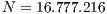In our approach, the Relabel operation is done globally using the distance to the destination node. This operation is done based on the nodes with available capacity to the destination . These nodes have a height equal to the height of the destination plus 1, . At first, the value of all nodes is equal to 1. On each iteration, nodes with available capacity to other nodes (previously marked) have a value of equal to the known height plus 1. Also, in subsequent iterations some nodes could be isolated from and only be connected to the source. This causes that the Relabel operation will not label these nodes.

Once the Relabel is performed on nodes which have excess and are isolated, they will never be able to send their excess and the algorithm will never stop. In order to solve this, the same idea must be applied but instead of using the node , it will use the source node . Thus, if a node has available capacity towards , then its height is calculated as . In Figure 4 there is an example of this operation. Figure 4(a) the heights of source and destination node are initialized. The height of the source node will be , where , and the height of the destination node is . Next, the algorithm updates the height values of the nodes according to their distance from the node , in Figure 4(b) the algorithm calculates the height of 8 nodes (with maximum height of 3). Note the 2 gray nodes which are isolated from the destination. Finally, in Figure 4(c), heights of the isolated nodes are calculated regarding to the distance to node .

One problem with this approach is that during the algorithm iterations, there are threads that do not execute any instructions. These threads are called inactive threads. To solve this, on each iteration it is necessary to create a container queue of nodes indexes that will run on the next iteration. It will only create the necessary threads to exploit the full capacity of the graphics hardware. Below an overview of the Push-Relabel algorithm on the GPU is shown:

1: 
2: 
3:  while  do
4: 
5: 
6: 
7:  end while

Line 1 shows an instruction that performs the operation as shown in Figure 4. The following statement performs the operation of , as explained at the beginning of this section. Even though there is an excess in any node in the graph, the algorithm proceeds to achieve the operation followed by the operation. The line 6, a queue of active nodes is created for the next iteration.

The function builds a linear array where threads indices are stored, which represents the active nodes in the graph to be used in the next iteration. Note that, the queue is completely stored on graphics hardware memory.

The following section shows a series of experimental results to test our approach.

5 Tests and Results

In order to test the effectiveness of our approach, we performed several tests of the segmentation to a set of volumes. The implementation was achieved under the Nvidia CUDA C programming language. The volume rendering was implemented using the library OpenGL^®;. Graphics hardware requires capability version 1.1 of CUDA.

We use an Intel i5 (3.20 GHz) with 4GB of RAM memory and a graphics card Nvidia GTX 470 with 448 CUDA cores (named ); and another computer with the same characteristic but with a graphics card Nvidia GTX 240 with 96 CUDA cores, named . The operating system was Microsoft Windows 7 64 bits. The sampling precision of volumes is 8 bits. Table 1 shows the characteristics of the volumes, and Figure 5 shows a simple render of the volumes.

Figure 5: Volume dataset used for our tests. All volumes were taken from http://www.volvis.org.

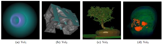
The first volume, Figure 5(a), represents a simulation of the spatial probability distribution of the electrons in a high potencial protein molecule. The Figure 5(b) is a CT scan of two cylinders of an engine block. Next, the third, Figure 5(c), is a simple CT scan of a bonsai tree. Finally, the Figure 5(d) is a MRI scan of a human head.

---

Table 1: Characteristics of the volumes used in tests.

---

Next, we present our experimental results for execution time, amount of space consumed, number of CUDA threads generated, comparison of visual results and comparison between the GPU and a CPU version of our approach.

5.1 Performance

In order to test the volume segmentation algorithm presented in this paper, we decided to implement two schemes: the sequential version based on CPU, and the parallel version based on GPU. For each volume, 3 different transfer functions were considered in the segmentation process. The first represents the identity function (), the second represents a function that helps to separate the voxels in foreground-background based on their intensities () and the third function was generated to highlight the interest object within the volume ().

When measuring the execution times it is possible to distinguish two main phases of the algorithm: First, the creation of the graph which occupies (in average) the of the total time of the algorithm execution. Secondly, the maximum flow algorithm completeness (which occupies the remaining).

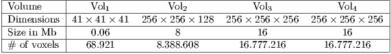
An important factor that affects directly the execution time (and the memory occupied) is the number of voxels inside the selection of the user, i.e. inside the sub-volume (purple cube in Figure 3). For instance, using the same sub-volume of selection and the volume Vol, the sequential version runs on and the parallel version runs on and over the cards and respectively. The reported times indicate that using the CPU is faster than using the GPU of the graphics card due to the volume dimension. Since Vol is small, the parallel version on the GPU considers the data transfer time from RAM to graphics memory. Table 2 shows a summary of the execution times obtained in our tests.

Thus, using a volume of greater dimension, such as the volume shown in the Figure 5(b), the execution times vary. It is important to note that times shown in Table 2 represent a time average using the three transfer functions. The composition of the transfer function influences directly over the running time of our approach, due to the number of iterations required to complete the maximum flow algorithm.

---

Table 2: Execution times obtained by each test volume.

---

According to the dimension of the sub-volume of selection, times can vary due to the influence of the number of threads created on the iterations of the algorithm.

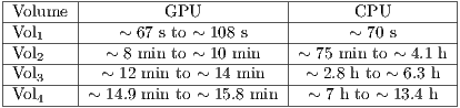
Furthermore, in order to measure the efficiency of the algorithm is necessary to consider the memory space used. More importantly, the graph construction is directly related to the existing number of voxels. For each voxel, different types of information such as connectivity, values of probabilities, and others should be stored. Then, a first approach to build the graph is to use all voxels which belong to the volume. This is not completely efficiently because the T-Links from the source are only connected to the voxels inside the sub-volume of selection. Moreover, voxels connected through T-Links whose value is the maximum possible are outside the sub-volume of selection. According to the GrabCut theory, if an excess arrive one of these nodes, they resend all the excess to the destiny. Thus, if a node inside the sub-volume of selection is connected to an outside node across a N-Link with value , the node has to send an excess towards , and this would send to the destination. It can be concluded that if a node is connected to another which is outside the sub-volume of selection, it causes the same effect that if a node is connected directly to the destination using T-Link with value equal to . For this reason, in this paper we only load voxels that are inside the selection volume in order to store in memory the relevant data to execute the algorithm.

Using the approach mentioned before, it can be noticed that connections from the source to the destination are performed using the nodes belonging to the sub-volume of selection. This gives us an efficient way to create the graph which will be processed by the minimal cut algorithm. This is because the area occupied by the sub-volume of selection will always be less (for a correct segmentation) than the total area occupied by the complete volume. This factor can be exploited to create only the necessary data structures and hence reduce the amount of memory used in the algorithm.

Table 3 shows a summary of the memory occupied by our algorithm selecting a particular case to the segmentation to each volume, with a sub-volume of selection which contains an object of interest.

---

Table 3: Memory occupied by each test volume.

---

Note that, the sub-volume of selection can not exceed the total amount of memory available in the graphics card. In the case of the graphics card , it supports a dimension up to 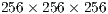voxels of the sub-volume.

5.2 Number of GPU Threads

When the algorithm starts, it runs a number of threads equal to the number of nodes in the graph. Following this statement in the subsequent iterations, the number of idle threads (without processing load) increases considerable making it an inefficient scheme. A thread is considered idle if it has no push or relabel operation in one iteration, or if it is identified in the background or foreground.

Our proposed approach, suggests the creation of a queue of active threads to store the next active thread on each iteration. The existence of an idle thread generates a load on the GPU for its creation, management and context execution which is unnecessary. Figure 6 shows an example of the number of threads generated in each iteration of the algorithm when it is applied to Vol and the three transfer functions (, and ) for an arbitrary selection of the volume. In the graph were taken only 56 of 359 iterations, because from the 56th iteration, the number of threads is considerably reduced until one working thread is reached.

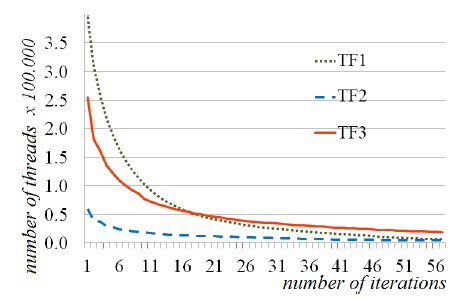
The graph shows the iterations from the 5th and forward. The first iteration presents 1 million of threads. For the 5th, the number of threads reach the 400.000, 60.000 and 254.000 for the , and respectively.A few iterations later, the number of threads decay dramatically to a few tens of threads, and the segmentation is performed.

5.3 Visual Results

As mentioned before, the tests consisted in applying three different transfer functions. For instance, for the Vol the test consisted in separating the ring, see Figure 5(a). Using the three transfer functions, and applying the same sub-volume of selection, an correct separation foreground/background was achieved.

The segmentation process to the Vol finds to separate two cylindrical pieces and two rings which exist within the engine volume. The results shows a good segmentation using the three transfer function. Particularly, with the the time obtained is less than using the other two due to its shape.

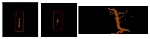
In the segmentation process of Vol, adequate results are achieved by applying the three transfers functions to separate the stem from the rest of the tree. However, with the 3 functions, the sub-volume obtained by the segmentation has voxels which belong to the land where the tree is planted. This is owing to the similarity of intensity and color of these with the stem of the tree. In Figure 7 it presents a selection of the user on the volume in the Vol applying the transfer function .

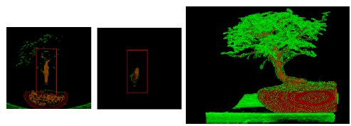
It can be noticed that the two first windows of the Figure 7 represent the selection made by the user in the direction of a coronal section plane (left) and transverse section plane (right). The final visual result of the segmentation is shown in Figure 8 where the final result is performed.

Figure 8: An example of the result of the segmentation of the Vol.

In volume Vol the goal is to segment the brain of the complete human head. Also, using the is generates more noise than the other 2 functions. This factor is caused by the small variation on the intensity between voxels of foreground and background. Nevertheless, the solution obtained shows small fragments of the cerebral cortex that should not be present. When using the transfer functions and , better results are obtained in spite of generating an unrealistic sub-volume according to the colors of the correct brain anatomy.

5.4 Comparison GPU and CPU

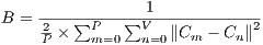
Using both version of the algorithm (sequential in the CPU and parallel on the GPU) it is possible to obtain different final visual results. For instance, the number of nodes presented in the GPU segmentation can vary with the number of nodes presented in the final graph using the CPU version. In the GPU, the order of updating the node excess modifies the graph in a different way that in the CPU. This is because a graph could have more than one minimal cut.

Figure 9 shows a comparison of both results. From a visual point of view, note that both reach a correct segmentation of the object of interest. Executing the algorithm on the GPU several times, it is possible to obtain different results. This is because there is no control over the execution order of threads. A method to prove these results consists in performing a comparison mechanism of the final results in order to manage the voxels segmented (e.g. difference between intensities voxels, heatmaps, and others).

6 Conclusions and Future Work

In this paper we presented a novel approach to the volume segmentation using the GPU. This approach was based on the GrabCut algorithm, originally presented to 2D image segmentation. The implementation of our algorithm was performed in two versions: a CPU-based sequential version and GPU-based parallel version under Nvidia CUDA. Tests performed showed excellent visual results when segmenting a volume in foreground and background.

The algorithm execution time and the final visual results after the segmentation are closely related to the size of the sub-volume selected by the user, and the transfer function used. If the sub-volume of selection occupies a considerable size according to the total volume dimension (assuming large volumes) then the number of active threads and nodes are also considerable. The transfer function determines the color of each voxel, if there are voxels with same color both inside and outside the selected area, the algorithm may classify certain foreground voxels as background voxels, and viceversa.

A limitation of the algorithm lies in the memory occupied by the graph and the data structures. This factor depends entirely on the selected GPU. In our tests, it is possible to segment any volume with the constraint of the sub-volume size. This can not be greater than voxels for our tests. Considering graphics cards with larger memory capacities, it is possible to handle larger volumes.

In the future we propose to apply and compare (in time and space) other minimum cut algorithms that can be parallelized efficiently on the GPU. At the same time, we will study the possibility to group voxels according to any color criteria to build a graph using ”super-nodes”. A super-node, groups a number of nodes ( node) to improve the execution time of the maximum flow algorithm on the GPU.

Acknowledgements

The authors would like to thank Prof. Walter Hernández for his valuable comments and insights.

References