


Services on Demand
Journal

Article
 English (pdf)
 Article in xml format
 Article references
Related links
Share

 Permalink
CLEI Electronic Journal
On-line version ISSN 0717-5000
CLEIej vol.16 no.3 Montevideo Dec. 2013
Abstract
Quantum computing proposes quantum algorithms exponentially faster than their classical analogues when executed by a quantum computer. As quantum computers are currently unavailable for general use, one approach for analyzing the behavior and results of such algorithms is the simulation using classical computers. As this simulation is inefficient due to the exponential growth of the temporal and spatial complexities, solutions for these two problems are essential in order to increase the simulation capabilities of any simulator. This work proposes the development of a methodology defined by two main steps: the first consists of the sequential implementation of the abstractions corresponding to the Quantum Processes and Quantum Partial Processes defined in the qGM model for reduction in memory consumption related to multidimensional quantum transformations; the second is the parallel implementation of such abstractions allowing its execution on GPUs. The results obtained by this work embrace the sequential simulation of controlled transformations up to 24 qubits. In the parallel simulation approach, Hadamard gates up to 20 qubits were simulated with a speedup of  over an 8-core parallel simulation, which is a significant performance improvement in the VPE-qGM environment when compared with its previous limitations.
Portuguese abstract:
A computação quântica propõe algoritmos quânticos exponencialmente mais rápidos do que seus análogos clássicos quando executados por um computador quântico. Devido a atual indisponibilidade de computadores quânticos para uso geral, uma abordagem para realizar a análise do comportamento e dos resultados de tais algoritmos é a simulação utilizando computadores clássicos. Uma vez que essa simulação é ineficiente devido ao crescimento exponencial das complexidades temporal e espacial, soluções para esses dois problemas são essenciais para a expansão das capacidades de simulação de qualquer simulador. Este trabalho propõe o desenvolvimento de uma metodologia definida por dois passos principais: o primeiro compreende a implementação sequencial das abstrações correspondentes aos Processos Quânticos e Processos Quânticos Parciais definidos no modelo qGM para redução no consumo de memória relacionado à transformações quânticas multidimensionais; a segunda é a implementação paralela dessas mesmas abstrações de forma a viabilizar sua simulação paralela através de GPUs. Os resultados obtidos por este trabalho contemplam a simulação sequencial de transformações controladas até 24 qubits. Na abordagem caracterizada pela simulação paralela, transformações Hadamard de até 20 qubits foram simuladas com um speedup de até 50x em comparação a uma simulação paralela com 8 cores, sendo uma significante melhora no desempenho do ambiente VPE-qGM quando comparado com duas limitações anteriores.
Keywords: Quantum Simulation, qGM Model, Quantum Process, GPU Computing.
Portuguese keywords: simulaçao quântica, computaçao GPU, simulaçao parallela .
Received: 2013-03-01, Revised: 2013-11-05 Accepted: 2013-11-05
Quantum Computing ( ) is a computational paradigm, based on the Quantum Mechanics (
 ), that predicts the development of quantum algorithms. In many scenarios, these algorithms can be faster than their classical versions, as described in [ 1] and [ 2]. However, such algorithms can only be efficiently executed by quantum computers, which are being developed and are still restricted in the number of qubits.
In this context, the simulation using classical computers allows the development and validation of basic quantum algorithms, anticipating the knowledge related to their behaviors when executed in a quantum hardware. Despite the variety of quantum simulators already proposed, such as [ 3 4, 5, 6, 7, 8, 9], the simulation of quantum systems using classical computers is still an open research challenge.
Quantum simulators powered by clusters have already been proposed in order to accelerate the computations, as can be seen in [ 6] and [ 7]. The downside of this approach is the need for expensive computing resources in order to build a cluster powerful enough to handle the computations associated with quantum systems described by many qubits. Moreover, a bottleneck generated by inter-node communication limits the performance of such simulators. Such statements motivate the search for new solutions focused on the modeling, interpretation and simulation of quantum algorithms.
The VPE-qGM (Visual Programming Environment for the Quantum Geometric Machine Model), previously described in [ 10] and [ 11], is a quantum simulator which is being developed considering both characterizations, visual modeling and distributed simulation of quantum algorithms. VPE-qGM presents the application and evolution of the simulation through integrated graphical interfaces. Considering the high processing cost of simulations, this work aims to improve the simulation capabilities of the VPE-qGM environment to establish the support for more complex quantum algorithms.
This work describes the improvements of the VPE-qGM’s simulation capabilities considering two approaches. The first is the implementation of the concepts of Quantum Process ( ) and Quantum Partial Process (
 ), in order to reduce the computation during the simulation. The second is the extension of its execution library to allow the use of GPUs to accelerate the computations.
This paper is structured as follows. Section 2 contains the background in quantum computing, GPU computing and some remarks on the VPE-qGM environment. Related works in three different approaches for quantum simulation are described in Section 3. The implementation of Quantum Processes and Quantum Partial Processes is depicted in Section 4. In Section 5, parallel quantum simulation on GPUs is described. Results are discussed in Section 6 together with a detailed analysis of sequential and parallel simulations for different types of quantum transformations. Conclusions and future work are considered in Section 7.
In order to understand and evaluate the contributions of this work, some concepts related to the two main areas (quantum computing and GPU computing) are discussed in the following subsections.
QC predicts the development of quantum computers that explore the phenomena of QM (states superposition, quantum parallelism, interference, entanglement) to obtain better performance in comparison to their classic versions [ 12]. These quantum algorithms are modeled considering some mathematical concepts.
In QC, the qubit is the basic information unit, being the simplest quantum system and defined by a unitary and bi-dimensional state vector. Qubits are generally described in Dirac’s notation [ 12] by
 | (1) |
The coefficients  and
and  are complex numbers for the amplitudes of the corresponding states in the computational basis (space states). They respect the condition
  , which guarantees the unitarity of the state vector of the quantum system, represented by
  .
.
The state space of a quantum system with multiple qubits is obtained by the tensor product of the state space of its subsystems. Considering a quantum system with two qubits,  and
and  , the state space consisting of the tensor product
  is described by
 | (2) |
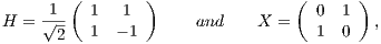
The state transition in a  -dimensional quantum system is performed by unitary quantum transformations defined by square matrices of order
  (i.e.,
  components since
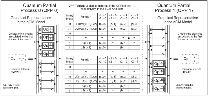
  is the number of qubits in the system). As an example, the matrix notation for Hadamard and Pauly X transformations are defined by
 |
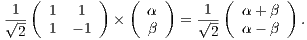
respectively. An application of the Hadamard transformation to the quantum state  , denoted by
  , generates a new global state as follows:
 |
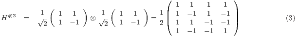
Quantum transformations simultaneously applied to different qubits imply in the tensor product, also named Kronecker Product, of the corresponding matrices, as described in (3).
Besides the multi-dimensional transformations obtained by the tensor product, controlled transformations also modify the state of one or more qubits considering the current state of other qubits in a multi-dimensional quantum state.
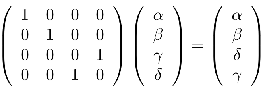
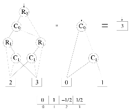
The CNOT quantum transformation receives the tensor product of two qubits  and
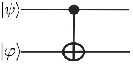
and  as input and applies the NOT (Pauly X) transformation to one of them (target qubit), considering the current state of the other (control). Figure 1(a) shows the matrix notation of the CNOT transformation and its application to a generic two-dimensional quantum state. The corresponding representation in the quantum circuit model is presented in Figure 1(b). Controlled transformations can be generalized (Toffoli) in a similar way [ 12].
By the composition and synchronization of quantum transformations, it is possible to execute computations exploring the potentialities of quantum parallelism. However, an exponential increase in memory space usually arises during a simulation, and consequentially there is a loss of performance when simulating multi-dimensional quantum systems. Such behavior is the main limitation for simulations based on matrix notation. Hence, optimizations for an efficient representation of multi-dimensional quantum transformations are required to obtain better performance and reduce both memory consumption and simulation time.
The GPGPU (General Purpose Computing on Graphics Processing Units) programming paradigm has become one of the most interesting approaches for HPC (High Performance Computing) due to its good balance between cost and benefit. For suitable problems, the high parallelism and computational power provided by GPUs can accelerate several algorithms, including the ones related to  .
.
The parallel architecture of the GPUs offers great computational power and high memory bandwidth, being suitable to accelerate many applications. The performance improvements are due to the use of a large number of processors (cores). The GPU’s architecture is composed by SMs (Streaming Multiprocessors), memory controllers, registers, CUDA processors and different memory spaces that are used to reduce bandwidth requirements and, hence, achieve better speedups.
The CUDA parallel programming model [ 13] provides abstractions such as threads, grids, shared memory space, and synchronization barriers to help programmers to explore efficiently all resources available. It is based on the C/C++ language with some extensions that allow the access of the GPU’s internal components. A program consists of a host-code and a device-code. The host-code runs on the CPU and consists of a non-intense and mostly sequential computational load. It is used to prepare the structures that will run on the GPU and eventually for a basic pre-processing phase. The device-code runs on the GPU itself, representing the parallel portion of the related problem.
Although the CUDA programming model is based on the C/C++ language, other languages and libraries are also supported. In the specific case of this work, the extension for the Python language, named PyCuda [ 14], was chosen over a lower-level, better-performance language due to two main reasons:
- Prototyping with the Python language results in a faster and easier development due to the low coding restrictions imposed;
- The host-code is comprised by methods for the creation of the basic structures that later are copied to the GPU. Such creation is based on string formatting and manipulation of multidimensional structures, which can be easily prototyped with Python. On the other hand, the device-code performs a more restricted and intensive computation, which is still implemented in the C language as a regular CUDA kernel.
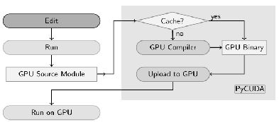
By using features of PyCuda such as garbage collection, readable error messages, and faster development, the technical part of the development processes becomes easier and greater attention is given to the algorithmic problem. A basic PyCuda workflow is shown in Figure 2. Binary executables are obtained from a C-like CUDA source code (CUDA kernel) generated by PyCuda as a string, allowing runtime code generation. The kernel is also compiled during runtime and stored in a semi-permanent cache for future reuse, if the source code is not modified.
The VPE-qGM environment is being developed in order to support the modeling and distributed simulation of algorithms from QC, considering the abstractions of the qGM (Quantum Geometric Machine) model, previously described in [ 15].
The qGM model is based on the theory of the coherent spaces, introduced by Girard in [ 16]. The objects of the processes domain  (see, e.g. [ 17, 18]) are relevant in the context of this work once they can define coherent sets that interpret possibly infinite quantum processes.
The qGM model substitutes the notion of quantum gates by the concept of synchronization of elementary processes (EPs). The memory structure that represents the state space of a quantum system associates each position and corresponding stored value to a state and an amplitude, respectively. The computations are conceived as state transitions associated to a spatial location, obtained by the synchronization of classical processes, characterizing the computational time unit. Based on the partial representation associated with the objects of the qGM model, it is possible to obtain different interpretations for the evolution of the states in a quantum system.
In the qGM model, an EP (elementary process) can read from many memory positions of the state space but can only write in one position. For example, the application  , described in (2.1), is composed by two classical operations:
 the normalization value
  is multiplied by the sum of the amplitudes of the two states and the result is stored in the state
  ;
;  the normalization value
  is multiplied by the subtraction of the amplitudes of the two states and the result is stored in the state
  .
.
A Quantum Process ( ) that represents the
  transformation is obtained when two EPs, associated to the operations described in
  and
and  , are synchronized. Such construction is illustrated in Figure 3. The parameters of the EPs define a behavior similar to the vectors that comprise the corresponding definition matrix. During the simulation, both EPs are simultaneously executed, modifying the data in the memory positions according to the behavior of the quantum matrix associated to the
  transformation, simulating the evolution of the quantum system.
The interpretation for the concept of  is obtained from the partial application of a quantum gate.Consider the gate
  , defined in (3). Each line (
 ) of the corresponding matrix in
  , where
  , is characterized by a
  with a computation defined in Eq.(4), where
  represents one element of
  , indexed by
  (line) e
  (column). Therefore, the synchronization of the
  , for
, for  , is the equivalent in the qGM model to the computation generated by the matrix
  .
.
 | (4) |
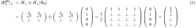
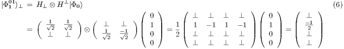
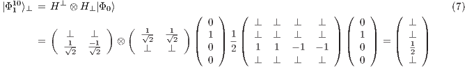
All possible subsets of EPs interprets different  . A
. A  corresponds to a matrix with a subset of defined components and a disjunct subset of undefined components (indicated by the bottom element
  ). Considering as context the elements of the computational basis
 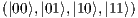 , it is possible to obtain a fully described two-qubit state
  by the union (interpreting the amalgamated sum on the process domain of qGM model) of four partial states, defined as follows from Eq. (5) to Eq. (8):
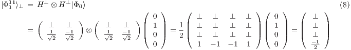
Hence, the state  is approximated by all states
  , with
 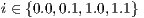 , resulting in the state
  .
.
Considering as context the values ( or
or  ) of the first qubit, the following partial states are obtained as in Eqs. (9) and (10):
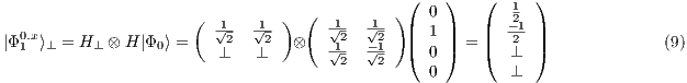
Now, the states  and
and  are other possible partial states of
  .
.
Although it is not the focus of this work, the qGM model provides interpretation for other quantum transformations, such as projections for measure operations.
Today, quantum simulators with different approaches are available. The most relevant are described in the next sections, representing the best solutions achieved so far for sequential and parallel simulation of quantum algorithms.
The QuIDDPro simulator proposed in [ 9] was developed in the C language and explores structures called QuIDDs (Quantum Information Decision Diagrams). QuIDDs are an efficient representation of multi-dimensional quantum transformations and states that are defined, in matrix notation, by blocks of repeated values. QuIDDs are capable of identifying such patterns and create simple graphs that represent data and assure low memory consumption and data access.
A QuIDD is a representation based on decision graphs, and computations are performed directly over this structure. For states with the same amplitude, an extremely simple QuIDD is obtained. For states with many different amplitudes, no compression can be reached. However, such states are not usual in QC.
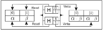
Quantum transformations and quantum states are represented as shown in Figure 4. The solid edge leaving each vertex assigns the logic value  to the corresponding bit that comprises the index of the desired state. The dashed edge assigns the logic value
  to its respective vertex. When a terminal node is reached, an index points to an external list that stores the amplitude generated by the values of each edge in the traveled path.
Results obtained by QuIDDPro are shown [ 19]. Instances of the Grover Algorithm up to  qubits were simulated, requiring
  KB of memory. Other simulation packages were limited to systems up to
  qubits. However, due to the sequential simulation,
  seconds were required.
3.2 Massive Parallel Quantum Computer Simulator
The Massive Parallel Quantum Computer Simulator (MPQCS) [ 6] is a parallel simulation software for quantum simulation. Simulations can be performed over high-end parallel machines, clusters or networks of workstations. Algorithms can be described through a universal set of quantum transformations, e.g. 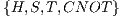 . Although these transformations can be combined in order to describe any quantum algorithm, such restricted set imposes limitations in the development process, since more complex operations must be specified only in terms of those transformations. However, this simplicity allows the application of more aggressive optimizations in the simulator, as computation patterns are more predictable.
Since the MPQCS explores the distributed simulation to improve the simulation, the MPI (Message Passing Interface) is used to communication. The downside of this approach is the overload of the interconnection system due to the large amount of data transfered during the simulation. As the interconnection is used to send data related to the state vector of the quantum system to the corresponding processing nodes, and such state vector grows exponentially, a high capacity interconnection is preferred.
The MPQCS simulator was executed on supercomputers such as IBM BlueGene/L, Cray X1E, and IBM Regatta p690+. The main results point to a simulation of algorithms up to  qubits, requiring approximately
  TB of RAM memory and
  processors.
In [ 20], the simulation of Shor’s algorithm was performed on the JUGENE supercomputer, factoring the number  into
into  . Such task required
  processors. The execution time and memory consumption were not published.
3.3 General-Purpose Parallel Simulator for Quantum Computing
The General-Purpose Parallel Simulator for Quantum Computing (GPPSQC) [ 7] is a parallel quantum simulator for shared-memory environments. The parallelization technique relies on the partition of the matrix of the quantum transformation into smaller sub-matrices. Those sub-matrices are then multiplied, in parallel, by sub-vectors corresponding to partitions of the state vector of the quantum system.
The simulator also considers an error model that allows the insertion of minor deviations into the definition of the quantum transformations ito simulate the effects of the decoherence in the algorithms.
By using the parallel computer Sun Enterprise (E4500) with  UltraSPARC-II (400MHz) processors,
  MB cache,
  GB of RAM memory and operational system Solaris 2.8 (
 bits), systems up to
  qubits were supported. The results containing the simulation time (expressed in seconds) required for Hadamard gates, from
  to
to  qubits are shown in Figure 5. Speedups of
  were obtained for a
  -qubit Hadamard transformation using
  processors.
3.4 Quantum Computer Simulation Using the CUDA Programming Language
The quantum simulator described in [ 8] uses the CUDA framework to explore the parallel nature of quantum algorithms. In this approach, the computations related to the evolution of the quantum system are performed by thousands of threads inside a GPU.
This approach considers a defined set of one-qubit and two-qubit transformations, being a more general solution in terms of transformations supported when comparing to the proposals of [ 6] and [ 7]. The use of a more expressive set of quantum transformations expands the possibilities for describing the computations of a quantum algorithm.
As main limitations of the quantum simulation with GPUs, memory capacity is the more restrictive one, limiting the simulation presented by [ 8] to systems with a maximum of  qubits. As an important motivation towards this approach, the simulation time can achieve speedups of
  over a very optimized CPU simulation.
4 Quantum Processes in the VPE-qGM Library
The execution library of the EPs, called qGM-Analyzer, contains optimizations to control the exponential growth of the memory space required by multi-dimensional quantum transformations [ 21]. These results showed a reduction in the memory space requested during the computations, simulating algorithms up to  qubits. However, this approach was still demanding a high computational time due to the exponential growth in the number of EPs executed.
The execution of EPs considers a strategy that dynamically generates the values corresponding to the components of the matrix associated with the quantum transformation being executed. Starting from these optimizations, this work extends the qGM-Analyzer in order to establish the support for the simulation of quantum transformations through  and
and  .
.
The main extensions consider the representation of controlled and non-controlled transformations, including all related possible synchronizations. The specifications of these and other new features are described in the following subsections.
4.1 Non-Controlled Quantum Gates
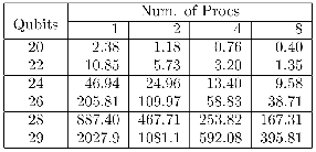
The  is able to model any multi-dimensional quantum transformation. Figure 6 shows a
  associated with a quantum system comprised of
  qubits (
 ), including its representation using EPs and the structure of such component in the qGM-Analyzer.
  stores the matrices associated with two-dimensional quantum transformations. Each line in
  is generated by the functions indicated in the second column of the
  . These functions (
 ,
,  and
and  ) describe the corresponding quantum transformation of the modeled application in the VPE-qGM.
The tuples of each line are obtained by changing the values of the parameters  and
and  . The first value of the tuple corresponds to the value obtained by the scalar product between the corresponding functions. The second indicates the column in which the value will be stored.
The matrix-order ( ) in
) in  is defined from the number of functions (
 ) grouped together. In Figure 6, the first matrix in
  , indicated by
  , has
, has  . Similarly,
  has
has  .
.
It is interesting that the order of each matrix in  can be arbitrarily determined but it is always consistent with the conditions for multi-dimensional quantum transformations. However, it is important to remember that when
  is large enough, e.g.
  , the memory consumption becomes a limitation. Hence, a balance between the order and the number of matrices in
  (
( ) interferes directly in the performance of the simulation.
Each line in all matrices in  has a binary index, a string with
  bits. For instance, in Figure 6, the index
  selects the first line of each matrix (
 from the first matrix and
  from the second matrix), allowing the computation of the associated amplitude to the first state of the computational basis of system (
 ).
).
Besides  , it is necessary to create a list (see (11)) containing auxiliary values for indexing the amplitudes of the state space, which must be multiplied by each values of the matrices in
  . In that list,
  indicates the total number of qubits in the quantum application.
![sizesList = [2q-n,2q-(2*n),...,2q-(|ML |*n)]](/img/revistas/cleiej/v16n3/3a03144x.png) | (11) |
The computation that results in the total evolution of the state vector of a quantum system is defined by the recursive expression in Eq.(12), considering the following notation:
 is the number of matrices in
  ;
;  is a base position (starting in
  ) for indexing the amplitudes of the states in the quantum system;
  indicates a matrix in
  (starting in
  );
);  is a line index
  of a matrix
  ;
;  is the order
  of a matrix
  ;
;  stores the
  ;
;  is the tuple indexed by
  ;
;  is the tuple indexed by
 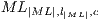 ;
;  is the amplitude of one state in the computational basis.
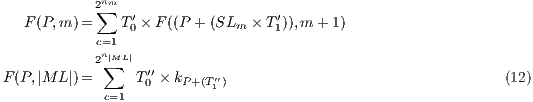
According to specifications of the qGM model, a  can be represented as a synchronization of
  . In this conception, it is possible to divide the
  described in Figure 6 in two
  , as presented in Figure 7.
  is responsible for the computation of all new amplitudes of the partial states in the subset
  of the computational basis and it is represented by the graphical component in the left side of the Figure 7. Similarly, on the right side, the graphical component associated to the
  is shown, computing the amplitudes in the subset
  of the computational basis independently from the execution of the
  .
.
 generated from the
  described in the Figure
 The  contribute with the possibility of establishing partial interpretations of a quantum transformation, allowing the execution of the simulation even in the presence of uncertainties regarding some parameters/processes. Therefore, in the local context of the computation of each QPP, it is possible to generate only a restricted subset of elements associated to a quantum gate. Complementary QPPs (that interpret distinct line sets) can be synchronized and executed independently (in different processing nodes). The bigger the number of QPPs synchronized, the smaller is the computation executed by each one, resulting in a low cost of execution.
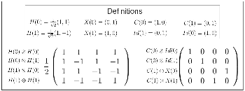
4.2 Definition of Controlled Quantum Gates
For non-controlled quantum gates, it is possible to model all the evolution of the global state of a quantum system with only one  . However, this possibility can not be applied to controlled quantum gates. The main difference can be seen in Figure 8, in which the following conditions are described:
- In the generation of the transformation
 , the expression (
 ) is maintained for all vectors, changing only the corresponding parameters;
 - In the description of the CNOT transformation, different expressions are required. This difference occurs due to the interpretation of the CNOT transformation.1
This interpretation can be extended to multi-dimensional transformations.
The complete description of the CNOT transformation is obtained by the expressions in Eq. (13), which defines a set of  called QPP_Set.
  for the CNOT transformation have their structures illustrated in Figure 9. The
  shown in Figure 9(a) and associated to
  describes the evolution of the states in which the state of the control qubit is
  (requiring the application of the Pauly X transformation to the target qubit). The evolution of the states in which the control qubit is
  is modelled by
  and generates the
  , illustrated in Figure 9(b). As these states are not modified, the execution of the
  is not mandatory.
 | (13) |
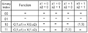 (a)  : change amplitudes : change amplitudes |
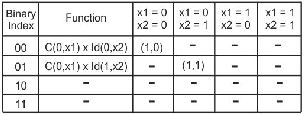 (b)  : do not change amplitudes : do not change amplitudes |
In general, 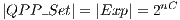 , where
  is the total number of control qubits in all gates applied. However, it is only necessary the creation/execution of the
  in a subset (QPP_Subset) of QPP_Set. If only one controlled gate is applied, then
 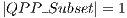 . When synchronization of controlled gates is considered,
  . As an example, consider the synchronization of two CNOT transformations shown in Figure 10(a). In this configuration, there are the following possibilities:
 e
e  : Apply X to
  and
and  ;
;  e
e  : Apply X to
  and Id to
  ;
;  e
e  : Apply X to
  and Id to
  ;
;  e
e  : Apply Id to
  and
and  .
.
In the VPE-qGM environment, this configuration is modelled using the expressions in (14). Hence,  . However, the
  , associated to the expression
  , does not change any amplitude in the system and should not be created/executed.

When controlled gates are synchronized with non-controlled gates (different from Id), all the amplitudes are modified. Therefore,  . The configuration illustrated in the Figure 10(b) is modelled through the expressions defined in (15). Now, two
  , identified by
  and
and  , respectively associated to the expressions in
  and
and  , are considered. However, it is not possible to discard the execution of the
  as it modifies the amplitudes of some states. Those changes are due to the H transformation, which is always applied to the last qubit, despite the control state of the CNOT transformation.
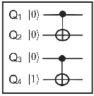 (a) Synchronization of CNOT gates |
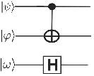 (b) Synchronization of the CNOT and H gates |
 | (15) |
After the creation of all necessary  , a recursive operator is applied to the matrices in
  for computing the amplitudes of the new state vector of the quantum system. This operator dynamically generates all values associated to the resulting matrix, originally obtained by the tensor product of the transformations, defining the quantum application.The algorithmic description of this procedure with some optimizations is shown in Figure 11.


![size(Matrices[matrixIndex])](/img/revistas/cleiej/v16n3/3a03237x.png)

![line← Matrices[matrixIndex][l][0];](/img/revistas/cleiej/v16n3/3a03239x.png)
![linePos← Matrices[matrixIndex][l][0];](/img/revistas/cleiej/v16n3/3a03240x.png)


![pos← basePos+ line[column][1];](/img/revistas/cleiej/v16n3/3a03243x.png)
![res← res+(partialV alue× line[column ][0]× memory[1][pos]);](/img/revistas/cleiej/v16n3/3a03244x.png)
![writePos← memP os+(linePos ×sizesList[matrixIndex]);](/img/revistas/cleiej/v16n3/3a03245x.png)
![res← res+memory[0][writePos];](/img/revistas/cleiej/v16n3/3a03246x.png)
![memory[0][writePos]← res;](/img/revistas/cleiej/v16n3/3a03247x.png)

![size(Matrices[matrixIndex])](/img/revistas/cleiej/v16n3/3a03249x.png)
![line← Matrices[matrixIndex][l][1];](/img/revistas/cleiej/v16n3/3a03250x.png)
![linePos← Matrices[matrixIndex][l][0];](/img/revistas/cleiej/v16n3/3a03251x.png)


![next_basePos← basePos+ (line[column][1]×sizesList[matrixIndex]);](/img/revistas/cleiej/v16n3/3a03254x.png)
![next_partialValue ←partialValue×line[column ][0];](/img/revistas/cleiej/v16n3/3a03255x.png)


![memPos+ (linePos×sizesList[matrixIndex]));](/img/revistas/cleiej/v16n3/3a03258x.png)
The execution cost of this algorithm grows exponentially when new qubits are added. Despite the high cost related to temporal complexity, it presents a low cost related to spatial complexity, once only temporary values are stored during simulation.
Considering all the features already included in the VPE-qGM environment, an important contribution of this work is the support for the simulation with GPUs.
This section describes the extension of the qGM-Analyzer library focused on the support for the parallel execution of  on a GPU. As such efforts are in their initial steps, only non-controlled transformations are considered for now.
The computation required by each CUDA thread comprehends the individual computation of  amplitudes of the new state vector of the quantum system.
For a generic  -dimensional quantum transformation, the number of CUDA threads are necessary is defined by
 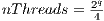 . Each block has the static configuration of
 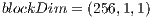 , Consequently, the grid is defined as
 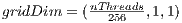 .
.
5.1 Constant-Size Source Matrices and Auxiliary Data
Following the specifications of the Section 4, a QPP is defined by building small-size matrices that are combined by an iterative function in order to dynamically generate the elements corresponding to the transformation matrix, which is obtained whenever the Kronecker Product between the initial matrices was performed. For the execution of a QPP, the system make use of the following parameters and all of them are stored in a NumPy ’array’ object:
- List of Matrices (matrices): matrices generated by the host-code;
- List of Positions (positions): position of an element in the corresponding matrix is necessary to identify the amplitude of the state vector that will be accessed during simulation;
- Width of Matrices (width): number of columns considering the occurrence of zero-values and the original dimension of the matrices;
- Column Size of Matrices (columns): number of non-zero elements in each column;
- Multiplicatives (mult): related to auxiliary values indexing the amplitude of the state vector;
- Previous Values (previousElements): number of elements stored in the previous matrices.
5.2 Allocation of Data into the GPU
When allocating structures into the GPU, data must be stored in the most suitable memory space (global memory, shared memory, constant memory and texture memory) to achieve good performance. As the QP parameters remain unchanged during an execution, they are allocated into the GPU’s constant memory. Such data movement is performed by PyCuda as described in the following steps:
- In the CUDA kernel, constant data is identified according with the following syntax:
![__device__ __constant__ dType variable[arraySize]](/img/revistas/cleiej/v16n3/3a03265x.png) ;
; - The device-memory address of variable is obtained in the host-code by applying the PyCuda call:
![address =kernel.get_global(′variable′)[0]](/img/revistas/cleiej/v16n3/3a03266x.png) ;
; - Data copy is also performed in the host-code in order to transfer the data stored in the host-memory to the device-memory address corresponding to variable. Such process is performed by the PyCuda call:
 .
.
Notice that dataSource is a NumPy [ 22] object stored in the host memory.
This procedure is done for all variables cited in the Subsection 5.1.
Furthermore, the host-code contains two NumPy ’array’ objects that store the current state vector (readMemory) and the resulting state vector (writeMemory) after the application of the quantum transformations. Additionally, the parameter writeMemory has all its positions zeroed before each step of the simulation. Next, the data related to readMemory and writeMemory are copied to the global memory space of the GPU. The following methods consolidate such process:
 is related to a NumPy array creation, with all its values equal to zero and resides in the host side. The desired current state is then manually configured.
  represents the copy of the current (input) state vector from the host-memory to the device-memory through a PyCuda call.
  is the new (output) state vector of the system, only created in the device side and initialized with all its values equal to zero by a PyCuda call.
The CUDA kernel is an adaptation of the recursive algorithm presented in Figure 11 to become an iterative procedure, as GPUs’ kernels may not contain recursive calls. As this kernel is inspired by the Kronecker Product, it operates over an arbitrary number of source matrices. Each CUDA thread has its own internal stack and iteration control to define the access limits inside each matrix.
The computation of each thread can be depicted in seven steps, described as follows.
Step  : Initialization of variables in the constant memory, which are common to all CUDA threads launched by a kernel.
  ,
,  and
and  are defined in runtime by the PyCuda interpreter. For text formatting purposes, this Subsection considers the symbol
  as a representation of the declaration
  .
.
![◇ cuFloatComplex matricesC [TOT AL_ELEMENT S]; ◇ int positionsC[T OTAL_ELEMENT S]; ◇ cuFloatComplex lastMatrixC[LAST_MAT RIX_ELEMENT S ]; ◇ int lastPositionsC[LAST_MAT RIX_ELEMENT S]; ◇ int widthC[STACK_SIZE + 1]; ◇ int multC[ST ACK_SIZE +1]; ◇ int columnsC[STACK_SIZE + 1]; ◇ int previousElementsC [STACK_SIZE +1];](/img/revistas/cleiej/v16n3/3a03277x.png)
Step  : Shared memory allocation and initialization are both performed by all CUDA threads within a block.
  is defined in run-time by the PyCuda interpreter, which in general will assume the value
  .
.
![__shared__ cuF loatComplex newAmplitudes[SHARED_SIZE ]; for (int i= 0; i< 4; i++ ){ ind= threadIdx.x× 4+ i; newAmplitudes[ind]=make_cuF loatComplex(0,0);} __syncthreads();](/img/revistas/cleiej/v16n3/3a03281x.png)
Step  : Definition of access limits of a matrix, determining which elements each CUDA thread will access depending on its id and resident block. The
  ,
,  and
and  arrays are local to each thread and help controlling and indexation of the elements of each matrix in
  and
and  . The
. The ![(thId& (widthC[c]- 1))](/img/revistas/cleiej/v16n3/3a03288x.png) operation is analogous to the module operation
operation is analogous to the module operation ![thId%widthC [c]](/img/revistas/cleiej/v16n3/3a03289x.png) but performed as a bitwise
but performed as a bitwise  that is more efficient in the GPU
![int thId= blockDim.x× blockIdx.x+threadIdx.x; for(int c=ST ACK_SIZE - 1; c>- 1; c- - ){ begin[c]= (thId&(widthC[c]- 1))× columnsC[c]; count[c]= begin[c]; end[c]= begin[c]+ columnsC[c]; thId= floorf((thId∕widthC[c]));}](/img/revistas/cleiej/v16n3/3a03291x.png)
Step  : Forwarding in matrices is analogously performed as a recursive step, providing the partial multiplications among the current elements according to the indexes in
  .
.
![while (ind< STACK_SIZE ){ position= positionsC [previousElementsC [ind]]; mod= (position+ count[ind])& (widthC [ind]- 1); readStack[top+ 1]=readStack[top]+ (mod ×multC[ind]); offset= previousElementsC[ind]; element= matricesC [offset+ count[ind]]; valueStack[top+ 1]= cuCmulf(valueStack[top],element); top+ +; ind ++;}](/img/revistas/cleiej/v16n3/3a03294x.png)
Step  : Shared memory writing is related to a partial update of the amplitude in the state vector.
![c=0; for(int j =0; j < 4; j+ +){ res= make_cuFloatComplex(0,0); for(int k= 0; k< columnsC[STACK_SIZE ]; k+ +){ mod= (lastP ositionsC [c]&(widthC[ind]- 1)) readPos= readStack[top]+mod; mult=cuCmulf(lastMatrixC[c],readMemory[readPos]); res= cuCaddf(res,mult); c++;} writePos= threadIdx.x× 4+j; partAmp1 = newAmplitudes[writePos]; partAmp2 = cuCmulf(res,valueStack[top]); newAmplitudes[writePos]= cuCaddf(partAmp1,partAmp2);}](/img/revistas/cleiej/v16n3/3a03296x.png)
Step  : Index changing in previous matrices generates the next values associated to the resulting matrix. This process will occur until all the indexes reach the last element of the corresponding line in all matrices.
![top- -; ind- -; count[ind]+ +; while(count[ind]== end[ind]{ count[ind]=begin[ind]; ind- - ; count[ind]++; top - -;}](/img/revistas/cleiej/v16n3/3a03298x.png)
Step  : Copy data from shared memory to global memory after all CUDA threads have finished their calculations.
![thId= blockDim.x× blockIdx.x +threadIdx.x; for (int i=0; i< 4; i+ +){ writePos= thId× 4+ i; readPos= threadIdx.x× 4+i; writeMemory[writeP os]= newAmplitudes[readPos];](/img/revistas/cleiej/v16n3/3a03300x.png)
The results of this work are divided into:
- Performance analysis considering the optimizations for the sequential simulation considering the concepts of
 and
and  . Benchmarks consisting in algorithms for reversible logic synthesis, based on controlled transformations, and case studies of Hadamard transformations are used;
 - Performance analysis of the parallel simulations of Hadamard transformations using GPUs.
In this work, the focus on Hadamard transformations as a benchmark is justified due to its high computational cost, representing the worst case for the simulation in the VPE-qGM once all the transformations are always applied to the global state of the system instead of following a gate-by-gate approach. By doing so, it is guaranteed that our solution is generic and can deal with classical, superposed and entangled states using the same algorithmic solution.
6.1 Sequential Simulation Results
For the validation and performance analysis of the sequential simulation of quantum algorithms using  and
and  in the VPE-qGM, two case studies were considered. The first consists of benchmarks, fundamentally composed by controlled gates, selected among ones available in [ 23]. This choice is justified by two main aspects:
- Availability of source code for generation of the algorithms;
- Quantum algorithms with many qubits and dozens/hundreds of gates.
The second considers Hadamard gates up to  qubits (
 ,
,  ,
,  and
and  ), for analysis of non-controlled gates.
The validation methodology considers, for each case study,  simulations. A hardware where the simulations were performed has the following main characteristics: Intel Core i5-2410M at 2.3 GHz processor, 4GB RAM and Ubuntu 11.10 64 bits.
Execution time and memory usage were monitored. The main performance comparison was made against the previous version of the qGM-Analyzer, which supports the simulation of quantum algorithms using EPs, considering the optimizations described in [ 21]. The main features of each algorithm and the results obtained are presented in Tables 1 and 2, where quantum algorithms up to  qubits were simulated.
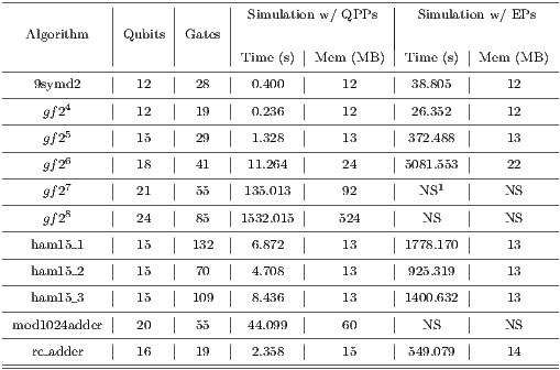
The memory consumption is similar in both versions of the library since optimizations for controlling the memory usage have already been added to the environment. As the optimizations regarding  and
and  only affect quantum gates, the high-cost of memory is due to the storage of state vector of the quantum system. The simulation time with both
  and
and  shows a time reduction when compared to the execution with EPs.
As presented in Figure 12(a), the simulation of controlled transformations using  showed a time reduction of approximately
  when compared to the simulation with EPs. Such performance improvement is due to the optimization focused on the identification of
  that changes any amplitude in the state space. Hence, only a subset of
  are executed, i.e., only part of the transformation is applied.
As an example, for each one of the  steps in the algorithm
  , only the operations corresponding to two vectors in a matrix of order
  are executed. Consequently, only a subset of the total number of amplitudes that contains the state of the quantum system is altered, requiring a smaller number of operations.
When the same algorithm is simulated using EPs, in each step of the simulation,  EPs are executed. In this approach, all amplitudes of the state space are recomputed, even though there are no changes in most values. Due to the exponential growth in the number of EPs, simulation of algorithms with more than
  qubits becomes unfeasible in this representation.
The algorithms  ,
,  and
and  were not included in Figure 12(a) because they are not supported by the older version of the qGM-Analyzer.
The percentage of time reduction for the simulation of Hadamard gates using  is shown in the Figure 12(b). In these cases, the improvement was not as significant as in the benchmarks with controlled gates, once that all the amplitudes of the state space are modified. Hence, both approaches result in the generation and computation over the elements associated to
  vectors. A reduction of
  in simulation time may be attributed to the generation of all elements in the same
  . In the EP approach,
  different components are executed, resulting in a larger number of operations.
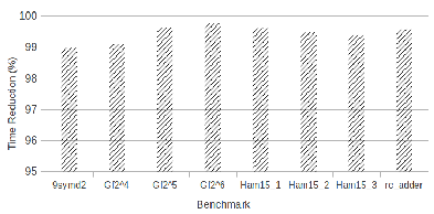 (a) Improvement percentage for the simulation with QPPs. |
 (b) Improvement percentage for the simulation of Hadamard gates with QPs. |
6.2 Parallel Simulation Results
The analysis of the parallel simulation using GPUs is based on the simulation of Hadamard transformations, always considering the global state of the quantum system. In order to compare the performance of this new proposal, the results of the parallel simulation obtained by the VirD-GM, which is detailed in [ 24], are used as reference once they represent the best performance for Hadamard transformations achieved in this project until now.
The parallel simulation was performed using a desktop with the following configuration: Intel Core i7-3770 CPU  GHz processor with hyperthreading,
  GB RAM, and Ubuntu
 bits. The execution algorithm presents the same complexity as the one depicted in the Figure 11 but it is implemented in Java. The methodology for the parallel simulation considers the execution of
  simulations of each instance of the Hadamard transformations, considering the simulation over
  ,
,  ,
,  , and
, and  cores.
For the simulation with GPUs, the tests were performed on the same desktop with a NVIDIA GT640 GPU. The software components are: PyCuda 2012.1 (stable version), NVIDIA CUDA 5 and NVIDIA Visual Profiler 5.0. There were simulated Hadamard transformations up to  qubits. The data to be analyzed, including the simulation time, was obtained with the NVIDIA Visual Profiler after
  executions of each application.
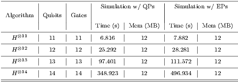
Table 3 contains the simulation time, in seconds, for Hadamard transformations ranging from  to to
to to  qubits, considering the parallel simulation by the VirD-GM and the parallel simulation using GPUs proposed in this work.
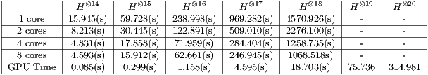
The results present a significant performance improvement when using a GPU. The standard deviation for the simulation time collected related to the simulation with the VirD-GM has reached a maximum value of  for the
  executed with
  cores. A complete
  -core simulation of the configurations with
  and
and  qubits would require approximately
  and
and  hours, respectively. Due to such elevated simulation time, those case studies were not simulated in the VirD-GM.
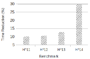
The speedups presented in Figure 13 have reached a maximum of  when comparing with the single core execution in the VirD-GM. The GPU-based simulation has outperformed the best parallel simulation in the VirD-GM by a factor of
  for the Hadamard of
  qubits running on
  processing cores. This improvement is explained by the number of CUDA cores available (384), as well as by its hierarchical memory architecture that allows a high data throughput. As the simulation performed by VirD-GM does not consider further optimizations regarding memory access and desktop computers were used, the performance obtained by the GPU execution was much better.
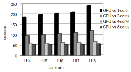
Applications with more than  qubits require at least
  processing cores for parallel simulation with the VirD-GM environment. For the simulation with GPUs, a
  -qubit Hadamard can be simulated with one mid-end device, such as a NVIDIA GT640.
Regarding the GPU’s execution, the NVIDIA Visual Profiler identified a local memory overhead associated with the memory traffic between the  and
and  caches, caused by global memory access corresponding to the reads in the
  variable, as described in Step 5 presented in Subsection 5.3.
The VPE-qGM environment introduces a novel approach for the simulation of quantum algorithm in classical computers, providing graphical interfaces for modelling and simulation of the algorithms.
The sequential simulation of quantum transformations (controlled or not) presented in this work reduces the number of operations required to perform state evolutions in a quantum system. The performance improvement, discussed in Section 6, allows the simulation of quantum algorithms up to  qubits.
In order to establish the foundations for a new solution to deal with the temporal complexity of such simulation, this work also describes an extension of the qGM-Analyzer library that allows the use of GPUs to accelerate the computations involved in the evolution of the state of a quantum system. The contribution of this proposal to the environment already established around the VPE-qGM is the first step towards a simulation of quantum algorithms in clusters of GPUs.
Although the support for simulation of quantum transformations using GPUs described in this work is in its initial stages, it has already significantly improved the simulation capabilities of the VPE-qGM. Elevated speedups, from  related to a 8-core parallel simulation to
  over the single core simulation, were obtained when comparing this novel solution to the simulation provided by the VirD-GM environment.
Simulations of Hadamard transformations up to  qubits were performed. Without the contributions of this work, such simulation may not be executed in the VPE-qGM or in the VirD-GM due to the elevated execution time. The Hadamard transformation was chosen as a case study in this work due to its high computational cost and represents the worst case for the simulation in this environment.
When comparing these results with related works, it is expected that other simulators will outperform our current solution due to two main reasons:
- Current solutions consider a universal set of quantum transformations, which is a restrict set of quantum operations that simplifies the optimizations for the simulation but imposes restrictions during the development of a quantum algorithm. Our solution consists of a generic approach in order to support any unitary quantum transformation;
- The data in the GPU’s global memory is often accessed. By moving sections of such data to the GPU’s shared memory and partitioning the computation of the CUDA threads in sub-steps to control memory access, performance can be improved.
An important consideration is that not only parallelization techniques are capable of improving performance. Future work also considers several algorithmic optimizations that will be applied to reduce the amount of computations, where the following ones can be highlighted:
- As the matrices that define quantum transformations are orthogonal, only the superior (or inferior) triangular may be considered in the computations. The most significant impact expected is the decrease of memory accesses and required storage. Reductions in the number of computations are also possible;
- A more sophisticated kernel that predicts multiplications by zero-value amplitudes of the state vector may avoid unnecessary operations. A major reduction in the number of computations is expected.
This work is supported by the Brazilian funding agencies CAPES and FAPERGS (Ed. PqG 06/2010, under the process number 11/1520-1), and by the project Green-Grid: Sustainable High Performance Computing (Ed. Pronex - Fapergs nb 008/2009, under process number 10/0042-8). The authors are grateful to the referees for their valuable suggestions.
[1] L. Grover, “A fast quantum mechanical algorithm for database search,” Proceedings of the Twenty-Eighth Annual ACM Symposium on Theory of Computing, pp. 212–219, 1996.
[2] P. Shor, “Polynomial-time algoritms for prime factorization and discrete logarithms on a quantum computer,” SIAM Journal on Computing, 1997.
[3] J. Agudelo and W. Carnielli, “Paraconsistent machines and their relation to quantum computing,” arXiv:0802.0150v2, 2008.
[4] A. Barbosa, “Um simulador simbólico de circuitos quânticos,” Master’s thesis, Universidade Federal de Campina Grande, 2007.
[5] H. Watanabe, “QCAD: GUI environment for quantum computer simulator,” 2002. [Online]. Available: http://apollon.cc.u-tokyo.ac.jp/ watanabe/qcad/
[6] K. D. Raedt, K. Michielsen, H. D. Raedt, B. Trieu, G. Arnold, M. Richter, T. Lippert, H. Watanabe, and N. Ito, “Massive parallel quantum computer simulator,” http://arxiv.org/abs/quant-ph/0608239, 2006.
[7] J. Niwa, K. Matsumoto, and H. Imai, “General-purpose parallel simulator for quantum computing,” Lecture Notes in Computer Science, vol. 2509, pp. 230–249, 2008.
[8] E. Gutierrez, S. Romero, M. Trenas, and E. Zapata, “Quantum computer simulation using the cuda programming model,” Computer Physics Communications, pp. 283–300, 2010.
[9] G. Viamontes, “Efficient quantum circuit simulation,” PhD Thesis, The University of Michigan, 2007.
[10] A. Maron, A. Pinheiro, R. Reiser, and M. Pilla, “Establishing a infrastructure for the distributed quantum simulation,” in Proceedings of ERAD 2011. SBC/UFRGS Informatics Institute, 2011, pp. 213–216.
[11] A. Maron, R. Reiser, M. Pilla, and A. Yamin, “Quantum processes: A new approach for interpretation of quantum gates in the VPE-qGM environment,” in Proceedings of WECIQ 2012, 2012, pp. 80–89.
[12] M. A. Nielsen and I. L. Chuang, Quantum Computation and Quantum Information. Cambridge University Press, 2000.
[13] NVIDIA, NVIDIA CUDA C Programming Guide. NVIDIA Corp., 2012, version 4.2.
[14] A. Kloeckner, “Pycuda online documentation,” 2012, http://documen.tician.de/pycuda/.
[15] R. Reiser and R. Amaral, “The quantum states space in the qGM model,” in Proc. of the III Workshop-School on Quantum Computation and Quantum Information. Petrópolis/RJ: LNCC Publisher, 2010, pp. 92–101.
[16] J.-Y. Girard, “Between logic and quantic: a tract,” in Linear logic in computer science, P. R. Thomas Ehrhard, Jean-Yves Girard and P. Scott, Eds. Cambridge University Press, 2004, pp. 466–471. [Online]. Available: http://iml.univ-mrs.fr/~girard/Articles.html
[17] R. Reiser, R. Amaral, and A. Costa, “Quantum computing: Computation in coherence spaces,” in Proceedings of WECIQ 2007. UFCG - Universidade Federal de Campina Grande, 2007, pp. 1–10.
[18] ——, “Leading to quantum semantic interpretations based on coherence spaces,” in NaNoBio 2007. Lab. de II - ICA/DDE - PUC-RJ, 2007, pp. 1–6.
[19] Q. C. Group, “Quiddpro: High-performance quantum circuit simulator,” 2007, disponível por WWW em <http://vlsicad.eecs.umich.edu/Quantum/qp/results.html> (dec.2011).
[20] M. Henkel, “Quantum computer simulation: New world record on jugene,” 2010, disponível em <http://www.hpcwire.com/hpcwire/2010-06-28/quantum_computer_simulation_new_world_record_on_jugene.html> (fev 2013).
[21] A. Maron, A. Ávila, R. Reiser, and M. Pilla, “Introduzindo uma nova abordagem para simulação quântica com baixa complexidade espacial,” in Anais do DINCON 2011. SBMAC, 2011, pp. 1–6.
[22] N. community, “NumPy user guide - release 1.6.0,” 2011, http://docs.scipy.org/doc/numpy/numpy-user.pdf.
[23] G. D. D. Maslov and N. Scott, “Reversible logic synthesis benchmarks page.” 2011, disponível por WWW em <http://www.cs.uvic.ca/ dmaslov>(apr.2012).
[24] A. Avila, A. Maron, R. Reiser, and M. Pilla, “Extending the VirD-GM environment for the distributed execution of quantum processes,” in Proceedings of the XIII WSCAD-WIC, 2012, pp. 1–4.

